Tutorial
Step 1: Create a PanPhaseField Project
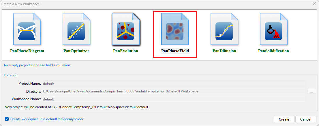
One can create a PanPhaseField project through menu “File → Create a New Workspace” or “File → Add a New Project” in an existing workspace. The “Module Window” pops out for user to choose a module for the new project as shown in Figure 1. Choose “PanPhaseField” module for phase-field simulation, and the PanPhaseField project will be created after user click on Create button or double click on the PanPhaseField icon.
Step 2: Load Thermodynamic and Mobility Database
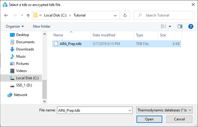
The next step is to load the database, which is “AlNi_Prep.tdb” in this example. Different from the normal thermodynamic database, this database also contains mobility data for the phases of interest in addition to the thermodynamic model parameters. Both are needed for carrying out phase-field simulation. By clicking the button ![]() on the toolbar, a popup window will open, allowing user to select the database file. User may select the TDB file and click on Open button or just double click on the TDB file to load it into the Workspace as shown in Figure 2.
on the toolbar, a popup window will open, allowing user to select the database file. User may select the TDB file and click on Open button or just double click on the TDB file to load it into the Workspace as shown in Figure 2.
Step 3: Load Phase-Field Database File
In addition to a combined thermodynamic and mobility database, a phase-field database (.pfdb) file which contains kinetic parameters for the alloy to be studied is also required for phase-field simulation.
A pfdb file is organized by the standard XML format, and a set of well-formed tags are deliberately designed to define phase-field model parameters for general and physical parameters of each phase.
In this example, the “AlNi_diffusion_only.pfdb” is prepared. This file can be opened by click ![]() button in the toolbar and be viewed in the Pandat™ workspace or through third-party external editors. The advantage to open this file in Pandat™ workspace is that all the key words will be highlighted which makes it easy to read. In this example, the matrix phase for this alloy is “Fcc”, which has one precipitate phase “L12_Fcc”. Phase field parameters, such as order parameter mobility and interface width, are defined in matrix.
button in the toolbar and be viewed in the Pandat™ workspace or through third-party external editors. The advantage to open this file in Pandat™ workspace is that all the key words will be highlighted which makes it easy to read. In this example, the matrix phase for this alloy is “Fcc”, which has one precipitate phase “L12_Fcc”. Phase field parameters, such as order parameter mobility and interface width, are defined in matrix.
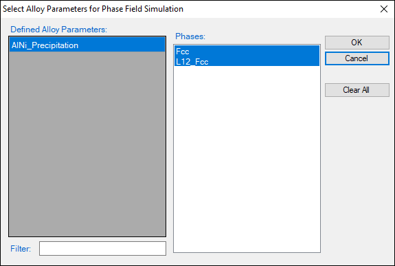
To load a phase-field database, user should navigate the command through menu "PanPhaseField → Load PFDB", or click icon ![]() from the toolbar. After AlNi.pfdb is chosen, a dialog box pops out automatically for user to select alloy and phases as shown in Figure 3. To select several phases at one time, for example in precipitation simulation where at least two phases should be selected, press and hold the <Ctrl> key.
from the toolbar. After AlNi.pfdb is chosen, a dialog box pops out automatically for user to select alloy and phases as shown in Figure 3. To select several phases at one time, for example in precipitation simulation where at least two phases should be selected, press and hold the <Ctrl> key.
Step 4: (Optional) Prepare VTK Files as Input Microstructure
PanPhaseField can use an input microstructure as initial condition. This is especially common when a digitized SEM picture or result from other simulation is used as initial condition. PanPhaseField follows standard VTK file format to load input microstructure. For example, in precipitation simulation, user can prepare a comprehensive VTK file containing order parameter of each phase and composition distribution. An example of this comprehensive VTK file is available in “input_2D_AlNi” of the example folder.
Please note that, the dimension in VTK file should be self-consistent, or an error message will popup when PanPhaseField tries to start a simulation. Please follow the examples in “input_2D_AlNi” to prepare VTK files as input.
Step 5: PanPhaseField Simulation
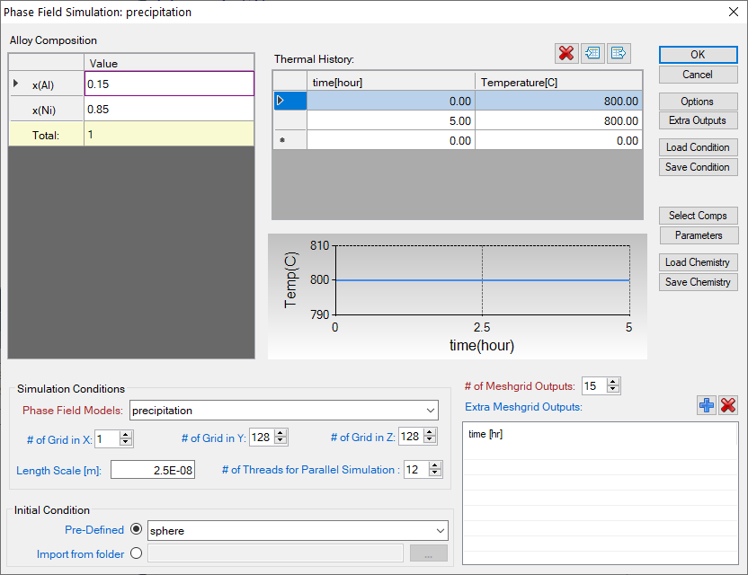
After successfully loading both thermodynamic/mobility and phase-field database file, and optionally the input VTK files, the phase-field simulation module is then being activated. To choose from Pandat™ GUI menu "PanPhaseField → Phase Field Simulation", or click icon ![]() from the toolbar. A dialog box entitled “Phase Field Simulation”, as shown in Figure 4, pops out for user’s inputs to set up the simulation condition: alloy composition, thermal history, and initial microstructure.
from the toolbar. A dialog box entitled “Phase Field Simulation”, as shown in Figure 4, pops out for user’s inputs to set up the simulation condition: alloy composition, thermal history, and initial microstructure.
-
Alloy Composition: User can set alloy composition by typing in or use the “Import from folder” function under “Initial Condition”. When “Import from folder” function is used, order parameters will also be loaded according to input files (VTK format).
-
Thermal History: Arbitrary heat treatment schedule can be set, with linear Time-Temperature relationship (i.e., constant cooling or heating rate) at each two consecutive rows. Time at the first row must be zero representing the initial time. The thermal history set up in Figure 4 represents an isothermal heat treatment for 5 hours at 800 °C. If the temperature in the two rows is different, it represents constant cooling or heating. Multi-stages of heat treatment can be set by adding more rows in the Thermal History column.
-
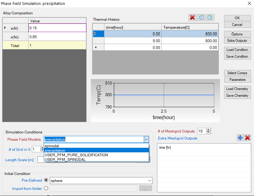
Phase Field Model: Select a built-in application or a user defined plugin. In Figure 5, “spinodal” and “precipitation” are built-in applications, at the same time user defined customized applications (plugins) are named “USER_PFM_XXX”.
-
Initial condition: phase field simulation must be initialized with a pre-existing microstructure without explicitly defining nucleation mechanism by a model. There are three Pre-Defined initial conditions: random, sphere, and empty. Random is used for spinodal decomposition simulation to apply randomized initial composition profile. Sphere is used for precipitation simulation applying a sphere particle with radius of 5 grids at the center of simulation box. Empty is used for simulation without explicitly initialize microstructure, for example, a nucleation simulation.
When “Import from folder” function is used, initial composition profile and/or initial order parameters following the data defined in VTK file(s) should be prepared before loading it.
-
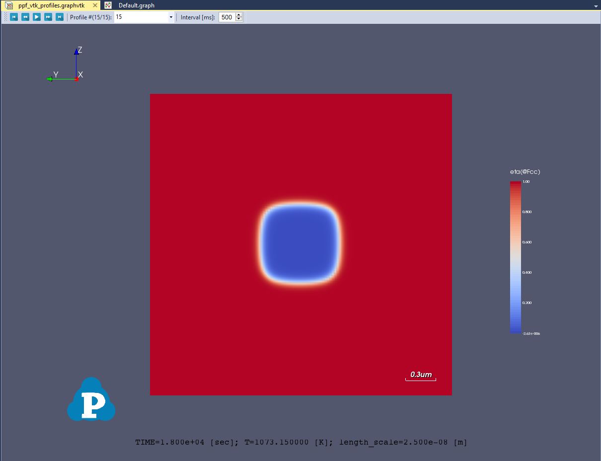
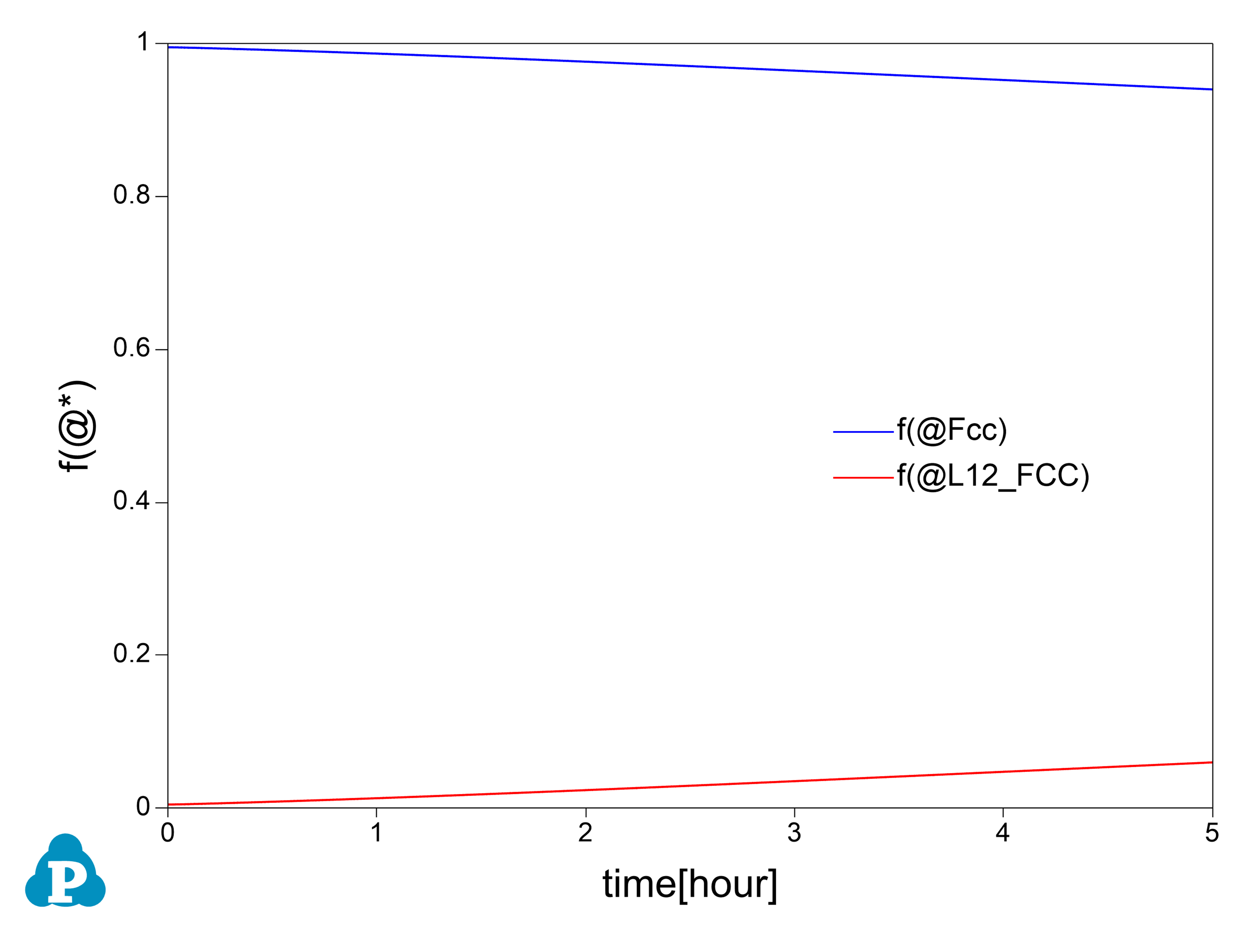
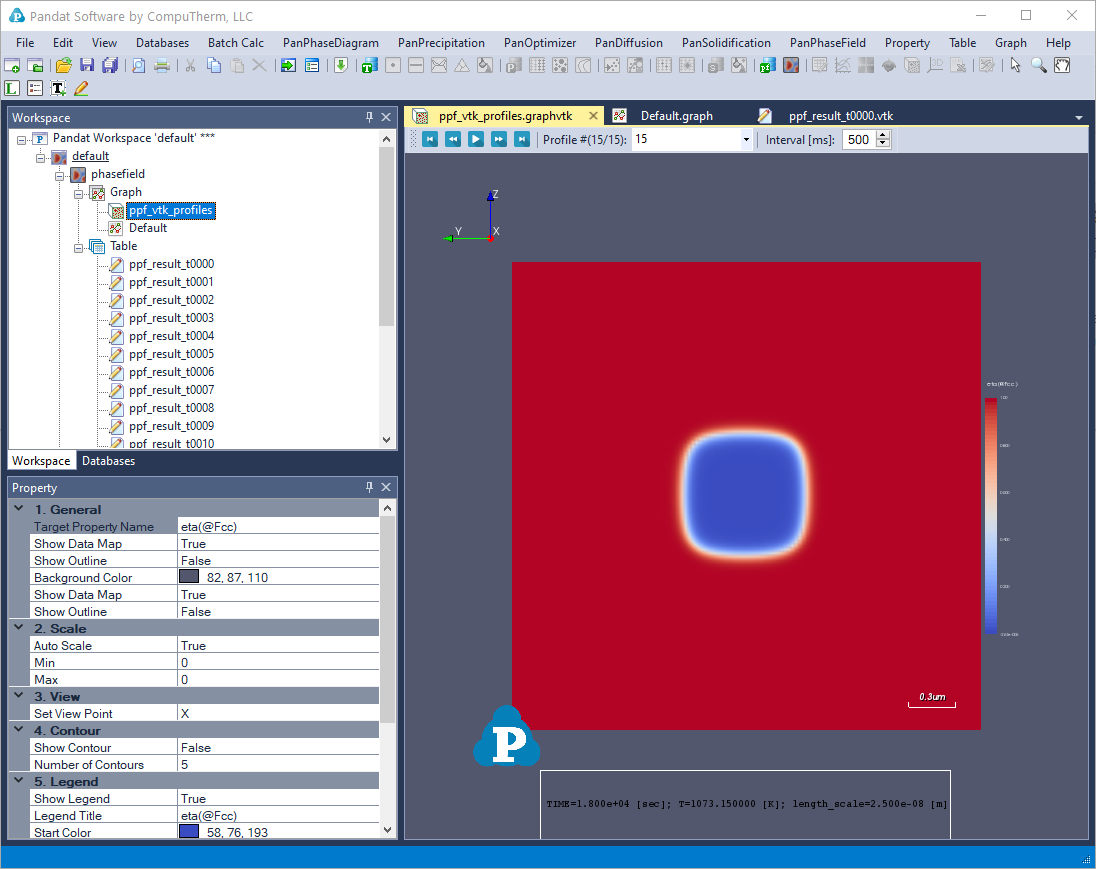
Run phase-field simulation: In Phase Field Simulation window (Figure 4), click OK to run the simulation. After the simulation is completed, its results are displayed in two types of formats in Pandat™ Explorer window: Graph and Table. By default, the graphs plotting microstructure and volume fraction of precipitate are shown in Figure 6 and Figure 7.
Step 6: Customize Simulation Results
Upon the completion of the phase-field simulation, a default table with related properties (such volume fraction) is automatically generated and a default graph is displayed in Figure 7.
However, it should be emphasized that, in addition to the default tables, variety of properties, such as temperature, nucleation driving force, nucleation rate, average composition of matrix phase can be retrieved through “Add a new table”.
Step 7: Add a New Table
To display other properties in addition to those listed in the Default table, add a new table function should be used through GUI.
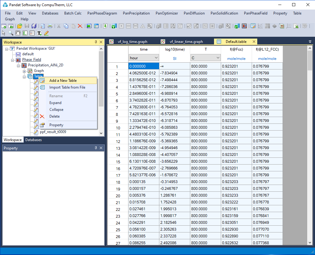
Add a new table function can be activated by the following ways: (1) selecting the “Table” node in the Explorer window, then right click the mouse and select “Add a New Table” option (as shown in Figure 8); or (2) choose “Add or Edit a Table” from the “Table” menu. This function allows user to create a new table at their own choices.
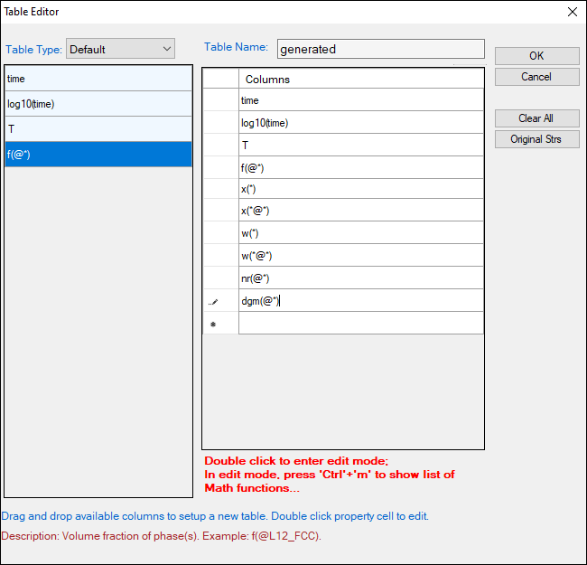
The basic layout of the window of “Add a new table” is shown in Figure 9. User can enter the available variables to the “Columns” field. The description of the available variables are listed in Table 1.
Step 8: Get VTK files
For the convenient of visualizing using third-party software such as ParaView, original VTK files of the phase-field simulation can be obtained by navigating to the Table folder follow the steps:
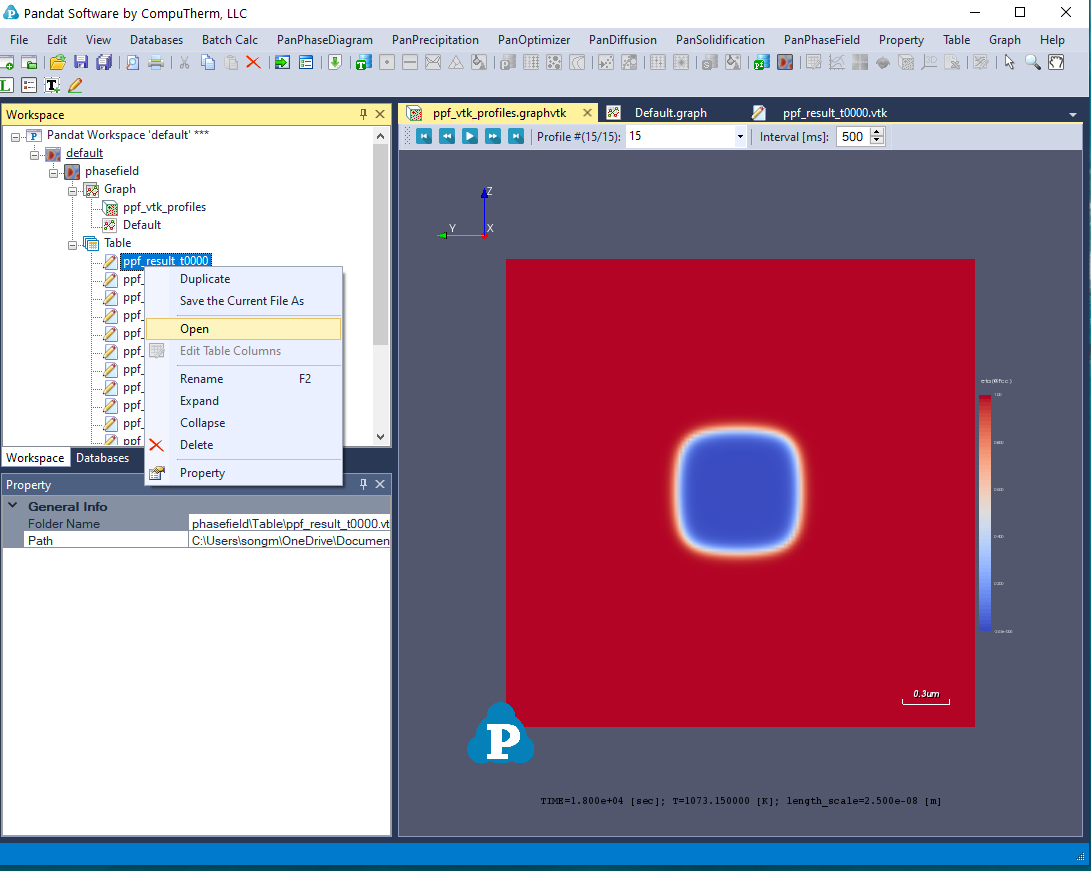
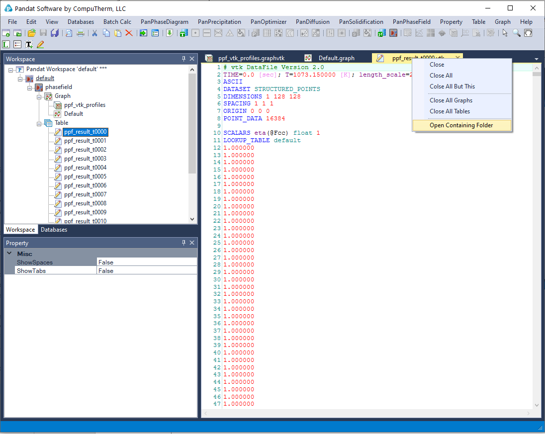
(1) Open any microstructure file in GUI window, as shown in Figure 10.
(2) “Open containing folder” which contains this microstructure file, as shown in Figure 11.
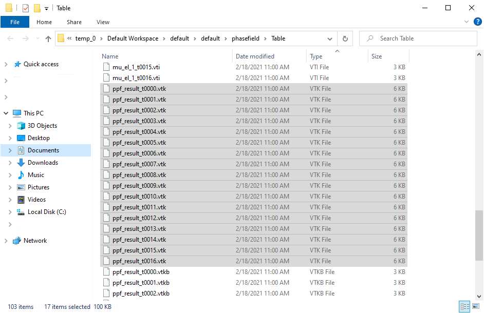
(3) Select all .VTK files for usage, as shown in Figure 12. (.VTKB all binary format of VTK files, which cannot be directly viewed by text editor, but can be opened by ParaVeiw)
Step 9: Load VTK files
Simulation results (VTK files) from batch mode (without using GUI) can be loaded to Pandat™ workspace for visualization. Users need to prepare two items to visualize VTK files in Pandat™ workspace:
(1) The batch file which describes the simulation performed in batch mode.
(2) The folder containing VTK files.
Batch file and VTK files must be consistent, for example they come from a same simulation. Follow the steps to load the VTK files:
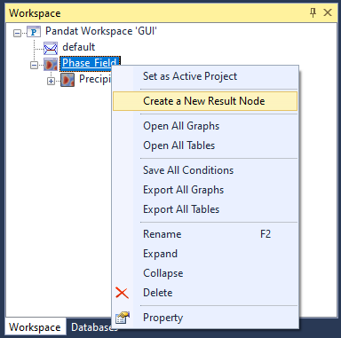
(1) Create a new result node in Pandat™ workspace.
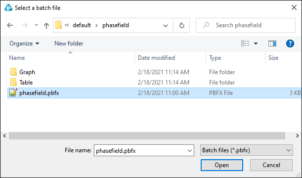
(2) Select a batch file for the batch mode calculation.
(3) Select corresponding VTK folder form the same batch mode calculation
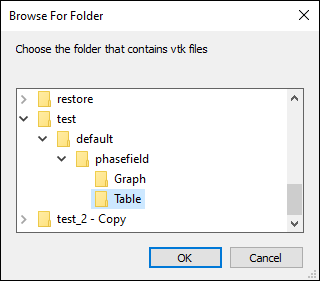
(4) After clicking OK in Figure 15, VTK files will be visualized.
Use a Plugin Defined by User
User-defined plugins can be loaded through Pandat GUI to perform a simulation using customer’s self-developed model.
Plugin should be organized inside “Pandat 2024/bin/PanPhaseField_Plugins” folder. Plugins inside this folder will be visible by PanPhaseField’s plugin viewer. Choose "PanPhaseField → Plugins", the Plugin viewer will show as in Figure 17.
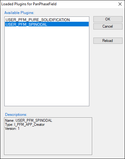
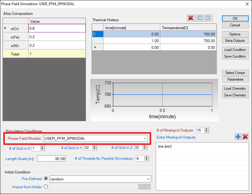
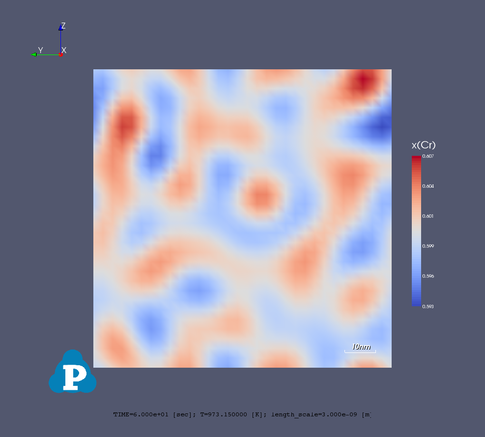
To perform a spinodal decomposition, follow Section Step 2: Load Thermodynamic and Mobility Database and Section Step 3: Load Phase-Field Database File to load the database files “FeCrNi.tdb” and “FeCrNi.pfdb” from “Pandat 2024 Examples/PanPhaseField/plugin_spinodal” folder. Set the condition and select UER_PFM_SPINODAL plugin from Phase Field Models, as is displayed in Figure 18. And the simulation result is displayed in Figure 19.