(1)

where R is the radius of the interface. R* is the radius of the critical nucleus and and are the row and column vector of the solute concentration difference between a (matrix phase) and β (precipitate phase), and [M] is the chemical mobility matrix. One can verify that the Eq. 1 can be further simplified and written as,

(2)

where K is the kinetic parameter, and is the transformation driving force defined as with being the molar chemical driving force and compensating the energy difference due to the Gibbs-Thompson effect.

(b) SFFK (Svoboda-Fischer-Fratzl-Kozeschnik) Model

The SFFK model [2004Svo] presents a set of linear equations describing the rate of change of radius and chemical composition of each precipitate in the system. Let the system consist of a matrix and a number of precipitates. The composition of each precipitate phase is not without boundary, it is determined by the complex lattice structure of the precipitate and the thermodynamic model used to describe the phase. The constraints can be written as,

(3)

where the parameters a_ij take on the values 0 or 1.

For the description of the state of a closed system under constant temperature and pressure, the state parameters q_i can be chosen. Then under several assumptions for the geometry of the system and/or coupling of process, the total Gibbs energy G of the system can be expressed by means of the state parameters, and the rate of the total Gibbs energy dissipation Q can be expressed by means of . In the case of Q being a positive definite quadratic form of the rates , the evolution of the system is given by the requirement of the maximum of the total Gibbs energy dissipation Q constrained by and by additional constrains which stem from the physical nature of the problem. Such a treatment is based on the thermodynamic extreme principle, which was formulated by Onsager in 1931 [1931Ons1, 1931Ons2].

Let μ₀i (i=1,...,n) be the chemical potential of component i in the matrix and μi (i=1,...,n) be the chemical potential ofcomponent i in the precipitate. All chemical potentials can be expressed as functions of the concentrations C_i. The total Gibbs energy of the system, G, is given by,

(4)

where σ is the interfacial energy and λ accounts from the contribution of the elastic energy and plastic work due to volume change of precipitates.

The evolution of the system corresponds to the maximum total dissipation rate Q and constrained where,

(5)

The problem can then be expressed by a set of linear equations. By solving the linear equation Ay=B, one can obtain the particle growth rate as well as the composition change rate of each precipitate phase. The detail description of the SFFK model can be found in reference [2004Svo].

(c) Morphology evolution

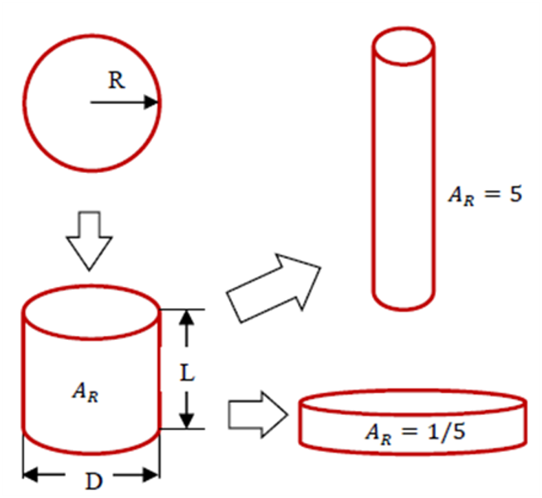
The driving force for the evolution of the aspect ratio of the precipitate stems from the anisotropic misfit strain of the precipitate and from the orientation dependence of the interface energy. The SFFK model was modified to account for shape factor and its evolution during precipitation process [2006Koz, 2008Svo]. In the model, the precipitate shape is approximated by a family of cylinders having a length L and a diameter D as shown in Figure 1. The aspect ratio A_R is used to describe the precipitate shape given by A_R = L/D. The quantity R is the equivalent precipitate radius of the spherical shape with the same volume of the cylindrical precipitate. With this definition, small values of A_R represent discs, whereas large values of A_R represent needles as shown in Figure 1.

In PanPrecipitation, the aspect ratio A_R of a precipitate phase can be treated as either a constant or a variable during evolution. In the former case, a set of shape factors are calculated based on A_R and the growth models are adjusted accordingly [2006Koz]. The shape factor S relating the surface of the cylindrical precipitate to the spherical precipitate is given by,

(6)

The shape factor K for interface migration of the precipitate is given by . The shape factor I for diffusion inside the precipitate is given by . The shape factor O for diffusion outside the precipitate is given by .

In the latter case, the original SFFK model was modified and the evolution equations are described by a set of independent parameters including the effective radius (R), mean chemical composition (C_ki) and the aspect ratio A_R of each precipitate phase. The evolution rates of these parameters , and are obtained by solving the linear equation Ay=B [2008Svo]. In the modified SFFK, the shape evolution is determined by the anisotropic misfit strain of the precipitate and by the orientation dependence of the interface energy. The total Gibbs energy of the system, G, is given by

(7)

The first term is the chemical part of the Gibbs energy of the matrix, the second term corresponds to the stored elastic energy and the chemical part of the Gibbs energy of the precipitates and the third term represents the total precipitate/matrix interface energy. The subscripts ‘‘0” denote quantities related to the matrix, e.g., N₀i is the number of moles of component i in the matrix and μ₀i is chemical potential in the matrix. The quantity λ_kA_R accounts for the contribution of elastic strain energy due to the volume misfit between the precipitate and the matrix and is calculated from Eq. 6.μ_ki are the values of chemical potentials in the precipitates corresponding to c_ki. In the model, there are two interface energies that must be assigned: at the mantle of the cylinder and at the bottom and top of the cylinder. The shape factor is obtained by calculating equivalent radius of a sphere with the same volume of cylinder.