Ni-14at.%Al precipitation simulation
In this tutorial, the Ni -14 at% Al alloy is taken as an example to demonstrate the functionalities provided by PanPrecipitation. The four files mentioned in this section (“AlNi_Prep.tdb”, “Ni-14Al_Precipitation.kdb”, “Ni-14Al_Exp.dat” and “Ni-14Al_Precipitation.pbfx”) can be found in the installation folder of Pandat™.
Step 1: Create a Workspace
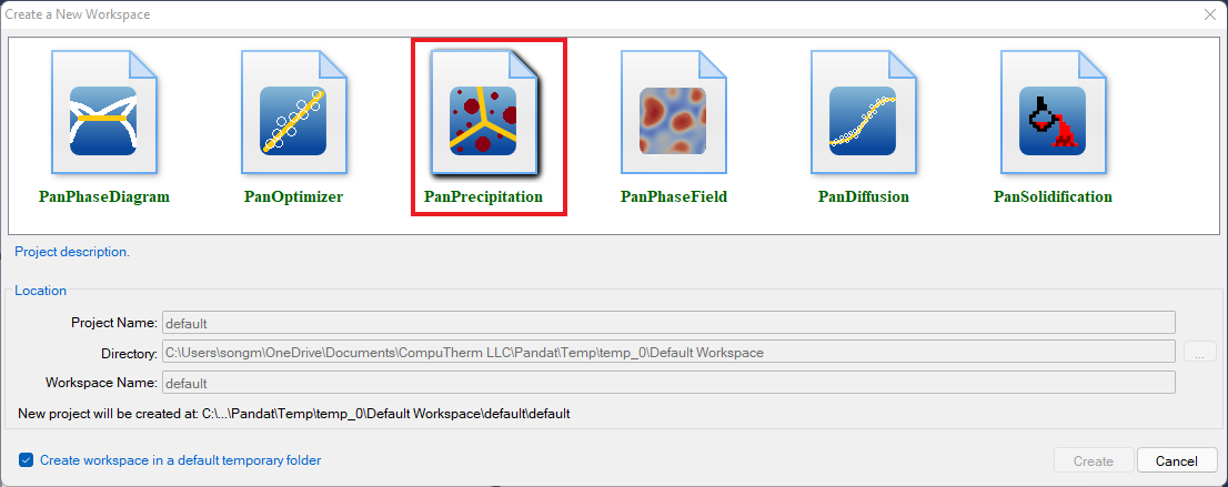
Let’s start this tutorial by “creating a workspace”. By clicking the ![]() button on the toolbar, the “Create a New Workspace” popup window will open. User can choose the “PanPrecipitation” icon and define the location (project name, directory and/or workspace name), then click the “Create” button to create a precipitation workspace. User can also create a default precipitation workspace by double-click the “PanPrecipitation” icon as shown in Figure 1.
button on the toolbar, the “Create a New Workspace” popup window will open. User can choose the “PanPrecipitation” icon and define the location (project name, directory and/or workspace name), then click the “Create” button to create a precipitation workspace. User can also create a default precipitation workspace by double-click the “PanPrecipitation” icon as shown in Figure 1.
Step 2: Load Thermodynamic and Mobility Database
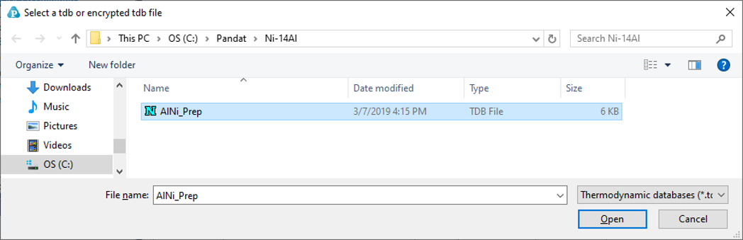
The next step is to load the database, which is AlNi_Prep.tdb in this example. Different from the normal thermodynamic database, this database also contains mobility data for the matrix phase (Fcc) in addition to the thermodynamic model parameters. Both are needed for carrying out precipitation simulation. By clicking the ![]() icon on the toolbar, a popup window will open, allowing user to select the database file. User may select the TDB file and click on Open button or just double click on the TDB file to load it into the PanPrecipitation module as shown in Figure 2.
icon on the toolbar, a popup window will open, allowing user to select the database file. User may select the TDB file and click on Open button or just double click on the TDB file to load it into the PanPrecipitation module as shown in Figure 2.
Step 3: Load Kinetic Parameters Database (KDB file)
A Kinetic Parameters Database (KDB file) is required for precipitation simulation. This file contains kinetic parameters which are alloy dependent. Each alloy is composed of one matrix phase and a number of precipitate phases. To organize these parameters in a more intuitive way, the standard XML format is adopted and a set of well-formed tags are deliberately designed to define the kinetic model (KWN or Fast_Acting) for each precipitate phase and its corresponding model parameters such as interfacial energy, molar volume, nucleation type, and morphology type.
In this example, the Ni-14Al_Precipitation.kdb is prepared. This file can be opened by click ![]() icon in the toolbar and be viewed in the Pandat™ workspace or through third-party external editors, such as NotePad, WordPad etc. The advantage to open this file in Pandat™ workspace is that all the key words will be highlighted which makes it easy to read. In this example, the matrix phase for this alloy is “Fcc”, which has one precipitate phase “L12_FCC”. The “KWN” model with “Sphere” morphology and “Modified Homogeneous” nucleation type are selected for precipitation simulation. There are five model parameters: Molar_Volume, Interfacial_Energy, Atomc_Spacing, Nucleation_Site_Parameter, and Driving_Force_Factor. These parameters have been developed for the Ni-14Al alloy in this particular example; these parameters need to be optimized for different alloys in terms of experimental data.
icon in the toolbar and be viewed in the Pandat™ workspace or through third-party external editors, such as NotePad, WordPad etc. The advantage to open this file in Pandat™ workspace is that all the key words will be highlighted which makes it easy to read. In this example, the matrix phase for this alloy is “Fcc”, which has one precipitate phase “L12_FCC”. The “KWN” model with “Sphere” morphology and “Modified Homogeneous” nucleation type are selected for precipitation simulation. There are five model parameters: Molar_Volume, Interfacial_Energy, Atomc_Spacing, Nucleation_Site_Parameter, and Driving_Force_Factor. These parameters have been developed for the Ni-14Al alloy in this particular example; these parameters need to be optimized for different alloys in terms of experimental data.
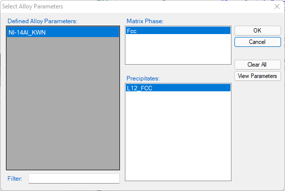
To load a KDB file, user should navigate the command through menu "PanPrecipitation→ Load KDB or EKDB", or click ![]() icon from the toolbar. After Ni-14Al_Precipitation.kdb is chosen, a dialog box pops out automatically for user to select the model, as shown in Figure 3, the “Ni-14Al_KWN” is chosen in this example. The Matrix Phase window allows user to select the matrix phase (Fcc in this case ) and the Precipitates window allows user to choose one or more precipitate phases of interest for simulation (L12_Fcc in this case). To select several phases at one time, press and hold the “Ctrl” key.
icon from the toolbar. After Ni-14Al_Precipitation.kdb is chosen, a dialog box pops out automatically for user to select the model, as shown in Figure 3, the “Ni-14Al_KWN” is chosen in this example. The Matrix Phase window allows user to select the matrix phase (Fcc in this case ) and the Precipitates window allows user to choose one or more precipitate phases of interest for simulation (L12_Fcc in this case). To select several phases at one time, press and hold the “Ctrl” key.
Click “View Parameters”, The “Create or Edit kdb Parameters” dialog as shown in Figure 1
Step 4: Precipitation Simulation
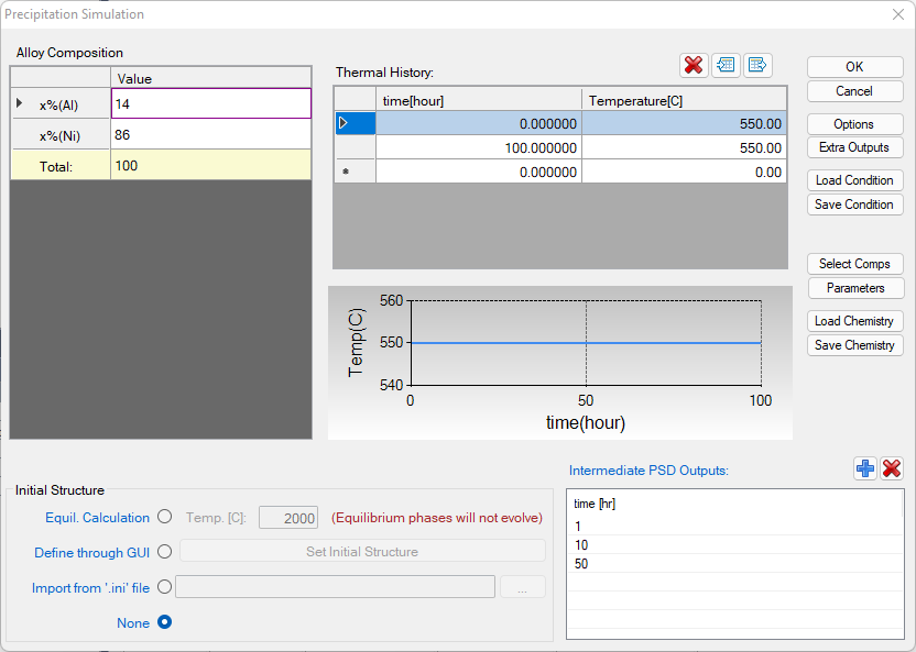
After successfully loading the thermodynamic and mobility database (TDB or PDB file) and Kinetic Parameters Database (KDB file), the function for precipitation simulation is then being activated. To perform a precipitation simulation, choose from Pandat™ GUI menu “PanPrecipitation → Precipitation Simulation”, or click ![]() icon from the toolbar. A dialog box entitled “Precipitation Simulation”, as shown in Figure 4, pops out for user’s inputs to set up the simulation conditions: alloy composition and thermal history.
icon from the toolbar. A dialog box entitled “Precipitation Simulation”, as shown in Figure 4, pops out for user’s inputs to set up the simulation conditions: alloy composition and thermal history.
-
Alloy Composition: User can set alloy composition by typing in or use the Load Chemistry function. User can also save the alloy composition through Save Chemistry. This is especially useful when working on a multi-component system, so that user does not need to type in the chemistry every time.
-
Thermal History: Arbitrary heat treatment schedule can be inputted, with a linear Time-Temperature relationship (i.e., constant cooling or heating rate) at each two consecutive rows. Time at the first row must be zero representing the initial time. The thermal history set up in the Figure 4 represents an isothermal heat treatment for 100 hours at 550 °C. If the temperatures in the two rows are different, it represents constant cooling or heating. Multi-stages of heat treatment can be set by adding more rows in the Thermal History column.
-
Set intermediate PSD outputs: Based on the specified intermediate PSD outputs, psd tables are automatically generated and the psd plot for the final time step will be created. As shown in Figure 4, the intermediate PSD outputs are set up at 1, 10, 50, and 100 hours, respectively.
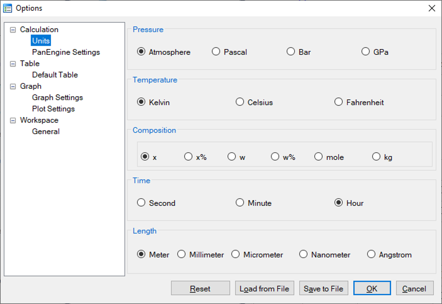
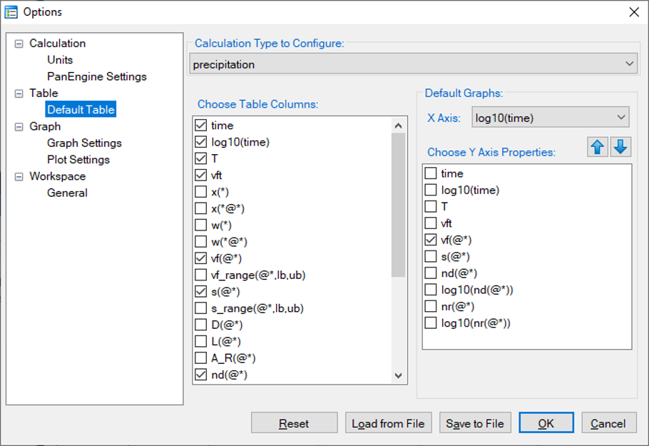
User can access the Options window by clicking the Options button. The Options window allows user to change the units for pressure, temperature, time and composition required in the simulation (as shown in Figure 5). User can also define the output Table and Graph within the Output Options window (as shown in Figure 6).
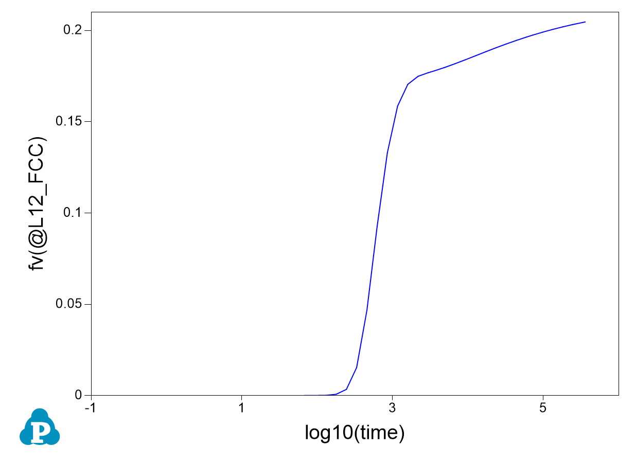
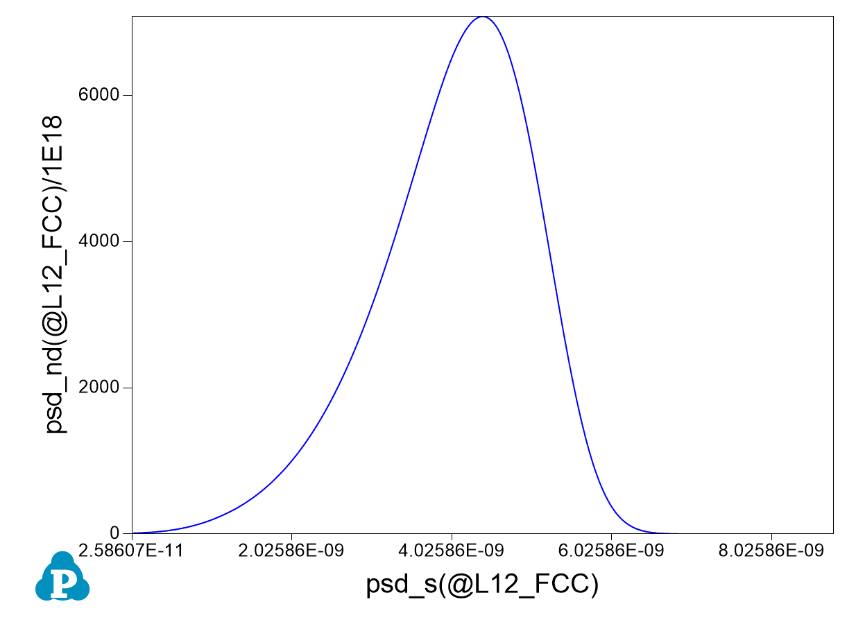
In Precipitation Simulation window (as shown in Figure 4), click OK to run the simulation. After the simulation is completed, its results are displayed in two types of formats in the Pandat™ Explorer window: Graph and Table. By default, the graphs plotting volume fraction evolution and PSD at 100 hours are displayed in the Pandat™ main window as shown in Figure 7 and Figure 8, respectively. To view detailed simulation results, user can switch from Graph view to Table View by clicking tabs in the Pandat™ Explorer window.
User can customize the output results with Pandat™ batch file. Experimental data may be imported as a separate table using the syntax below:
<table source="Ni-14Al_Exp.dat" name="exp"/>
The experimental data file should be in the same folder where the batch file locates, otherwise a full path is needed for the experimental file as shown below:
<table source="D:\Pandat\Precipitation\Ni-14Al_Exp.dat" name="exp"/>
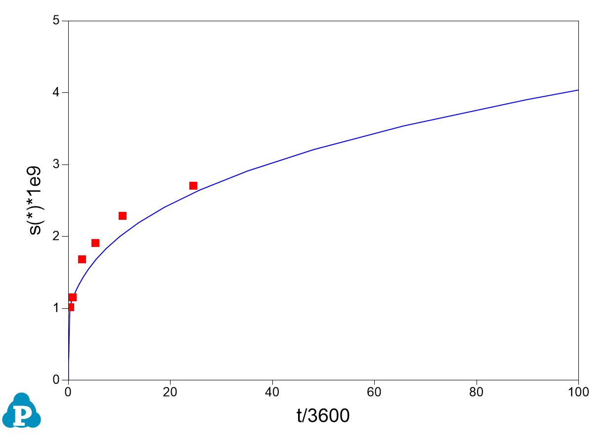
And the experimental data can be plotted together with the calculated results using the syntax below to obtain a diagram as shown in Figure 9.
<graph name="size">
<plot table_name="default" xaxis="t/3600" yaxis="s(*)*1e9"/>
<plot type="point" table_name="exp" xaxis="t(hr)" yaxis="radius(nm)"/>
</graph>
Step 5: Customize Simulation Results
As all other calculations available in Pandat™, upon the completion of the precipitation simulation, a default table with related kinetic properties (such as time, total transformed volume fraction, average size of each precipitate phase, number density of each precipitate phase and nucleation rate of each precipitate phase) is automatically generated and a default graph for volume fraction changes is displayed Figure 7.
However, it should be emphasized that, in addition to the default tables, variety of properties, such as temperature, volume fraction of each individual precipitate phase, instant composition of matrix phase and also size distribution related information if the KWN model is used for simulation, can be retrieved through “Add a new table”. Symbol and syntax for retrieving quantities of matrix phase, precipitate phases or grain are listed in Table 9.
Add a New Table
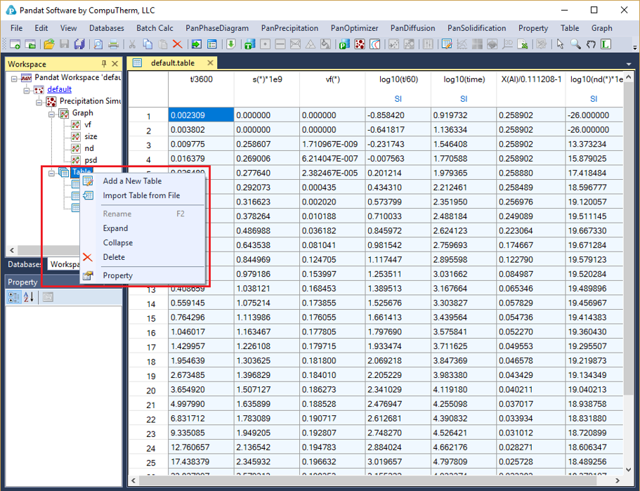
“Add a new table” function can be activated by the following ways: (1) selecting the “Table” node in the Explorer window, then right click the mouse and select “Add a New Table” option (as shown in Figure 10); or (2) choose “Add or Edit a Table” from the “Table” menu. This function allows user to create a new table at their own choices.
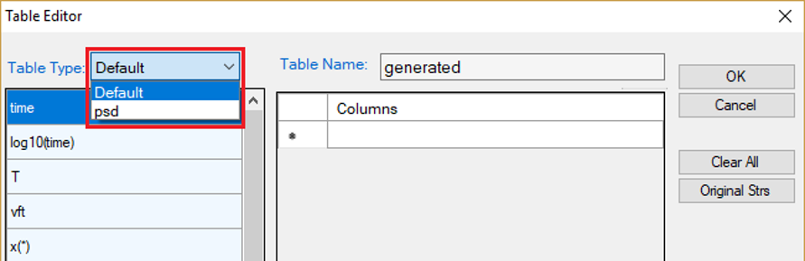
The basic layout of the window of “Add a new table” is shown in Figure 11. There are two major parts in this window. The left part is the available variables and contents. User first chooses the type of the tables from the “Table Type” drop-down list as highlighted in Figure 11, to show the list of available variables. The right part is the generated table field. User can drag the available variables from the left column to the right side by clicking and holding the left mouse button.
Table Format Syntax
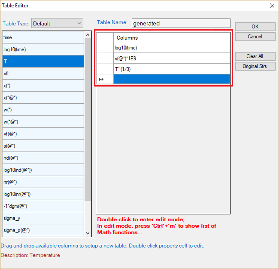
Moreover, mathematical calculation over these properties is allowed in PanPrecipitation. Accordingly, a variety of property diagrams can be generated based on the customized tables, which offers users an excellent flexibility for different applications. A detailed description of table format is given below. Figure 12 shows the dialog window of table editor for customized new table. The symbol “*” can be used to get quantities of all the phases or all components. As an example, s(*) retrieves the average size of phase L12_FCC, which is equivalent to s(L12_FCC).
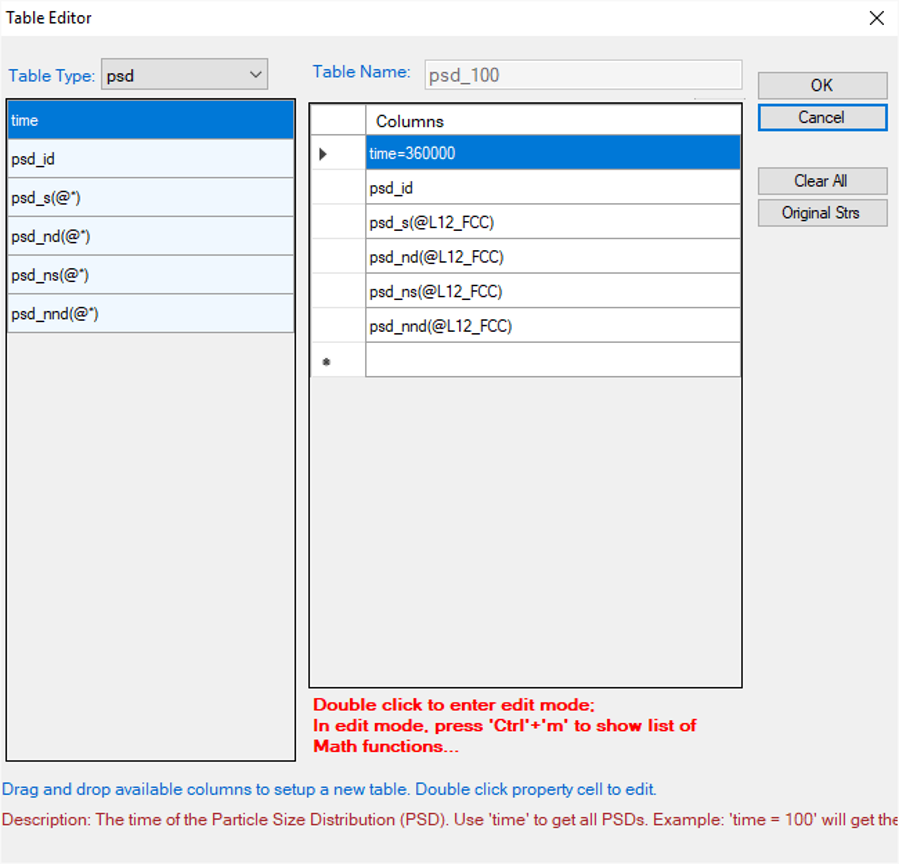
Figure 13 shows the dialog window of table editor for user to get a psd table by specifying time. For example, the psd table at 100 hours can be obtained by setting “time = 360000”. Note that the default unit for time is second.