Thermal Resistivity and Thermal Conductivity
Thermal conductivity of a pure element or a stoichiometric phase at temperature above 273 K is described as a function of temperature using the following equation:
where k is the thermal conductivity and T is the temperature in Kelvin. This function can reasonably fit most of the experimental thermal conductivity data of elements at temperature above 273 K.
The thermal conductivity of a solid solution phase can be calculated from thermal resistivity, which is the reciprocal of thermal conductivity. According to the Nordheim rule, the thermal resistivity ( ρ ) of a solid solution phase can be described by the following Redich–Kister polynomials:
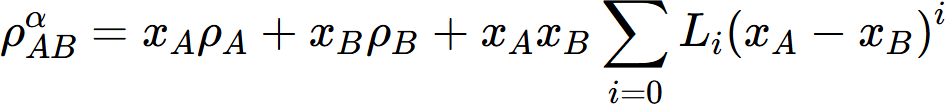
where  is the thermal resistivity of the a solution phase in the A-B system. xj and rj are the mole fraction and thermal resistivity of pure elements j, respectively. Li are the ith order interaction parameters which are used to describe the effect of solute elements on the thermal resistivity. In general, the interaction parameter can be expressed as:
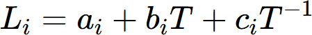
where the parameters ai, bi and ci are evaluated based on the experimental data.
In real alloys, multiple phases coexist, influencing the overall thermal conductivity. The thermal conductivity is affected by the volume fraction and morphology of these phases. The series and parallel models are fundamental theoretical approaches for two-phase composites, representing phase arrangements perpendicular and parallel to the heat flow direction, respectively. These models establish the lower and upper bounds of the effective thermal conductivity, expressed as:
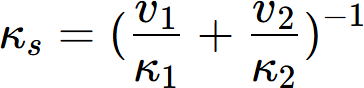
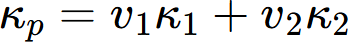
where κs and κp represent the effective thermal conductivities of an alloy with two-phase microstructure under series and parallel model, and v1, v2, κ1 and κ2 represent volume fractions and thermal conductivities of the two phases, respectively.
Pandat provides System_Property definition to automatically calculate a system property based on a multi-phase structure. The thermal conductivities of an alloy with multiphase microstructure under series model and parallel model can be formulated as
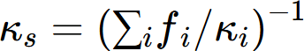
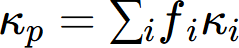
where fi, and κi represent molar fraction and thermal conductivity of the phase i, respectively.
Helsing et al. [1991Hel] proposed the effective thermal conductivity of lamellar eutectic microstructure relates to series and parallel models.
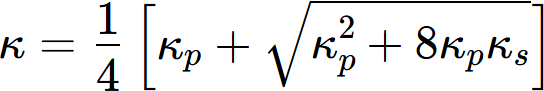
And the effective thermal conductivity of an alloy with multiphase microstructure can be calculated using Eq. 9.32-Eq. 9.34.
Due to the limited amount of experimental data available in literature, a default value (100W/mK) is set for those phases without data to avoid empty result of property calculation.
In this example, thermal resistivity of the Al-Mg binary alloys is described using the User-Defined Property function.
As shown in the AlMg_ThRss.tdb, the thermal resistivity ThRss is first defined as a user-defined property with a fixed default value since it hasn’t been pre-defined in the current Pandat software.
Function ThRss_default 298.15 0.01; 6000 N !
Type_Definition z PHASE_PROPERTY ThRss 1 !
As is seen, the thermal resistivity of the Liquid phase, Fcc phase or the Hcp phase follows the same format as that of Gibbs energy (Redlich-Kister formula) for a disordered solution phase.
Parameter ThRss(Liquid,Al;0) 298.15 1/ThCond_Al_Liq; 3000 N !
Parameter ThRss(Liquid,Mg;0) 298.15 1/ThCond_Mg_Liq; 3000 N !
Parameter ThRss(Fcc,Al;0) 298.15 1/ThCond_Al_Fcc; 3000 N !
Parameter ThRss(Fcc,Mg;0) 298.15 1/ThCond_Mg_Hcp; 3000 N !
Parameter ThRss(Fcc,Al,Mg;0) 298.15 0.02566-1.3333e-05*T+14.5*T^(-1); 3000 N !
Parameter ThRss(Hcp,Al;0) 298.15 1/ThCond_Al_Fcc; 3000 N !
Parameter ThRss(Hcp,Mg;0) 298.15 1/ThCond_Mg_Hcp; 3000 N !
Parameter ThRss(Hcp,Al,Mg;0) 298.15 0.0214-1.3669e-5*T+12.7158*T^(-1); 3000 N !
Parameter ThRss(Hcp,Al,Mg;1) 298.15 0; 3000 N !
Parameter ThRss(Hcp,Al,Mg;2) 298.15 0.14825-7.7706e-05*T+25.3031*T^(-1); 3000 N !
Thermal resistivity of the intermetallic phases with narrow solid solubility range in the phase diagrams is treated like a stoichiometric compound phase, i.e., the property is composition independent and irrelevant to its sublattice model/size (The parameter always refers to one mole of atoms.). It can be described as below:
Parameter ThRss(AlMg_Beta,*;0) 298.15 1/42; 6000 N !
Parameter ThRss(AlMg_Eps,*;0) 298.15 1/42; 6000 N !
Parameter ThRss(AlMg_Gamma,*;0) 298.15 -0.03267+2.7412e-05*T+20.722*T^(-1); 6000 N !
When the thermal conductivity of an intermetallic phase varies with composition, two possible definitions are available for the user to choose. The property can be expressed as a function of mole fractions of elements regardless of its original sublattice model used for those phases whose properties smoothly change with respect to composition. The thermal resistivity of the phase AlTi3 with a sublattice model of (Al,Ti)1(Al,Ti)3 is shown as an example below. The values of end members are set as one mole of atoms and not related to sublattice size. The property is calculated using phase composition (mole fractions of elements) and those property parameters defined similarly to that of the solution phase.
Parameter ThRss(AlTi3,Ti;0) 298.15 1/ThCond_Ti_Hcp; 3000 N !
Parameter ThRss(AlTi3,Al;0) 298.15 1/ThCond_Al_Fcc; 3000 N !
Parameter ThRss(AlTi3,Al,Ti;0) 298.15 0.1+110*T**(-1); 3000 N !
The other definition is expressed as a function of site fractions due to the sharp property variations related to site fractions change. The thermal resistivity of the phase B2 with a sublattice model of (Al,Ni)1(Ni,Va)1 is shown as an example below. The values of end members are defined with respect to sublattice size (total moles of atoms in all sublattices). The property is calculated using the site fractions of elements in each sublattice and those property parameters defined similarly to the Gibbs energy for the CEF model.
Parameter ThRss(B2,Al:Va;0) 298.15 +1/ThCond_Al_Fcc; 3000 N !
Parameter ThRss(B2,Al:Ni;0) 298.15 +2*(0.013-5e-7*T); 3000 N !
Parameter ThRss(B2,Ni:Ni;0) 298.15 +2/ThCond_Ni_Fcc; 3000 N !
Parameter ThRss(B2,Ni:Va;0) 298.15 +1/ThCond_Ni_Fcc; 3000 N !
Parameter ThRss(B2,Al,Ni:Ni;0) 298.15 0.5; 3000 N !
Parameter ThRss(B2,Al:Ni,Va;0) 298.15 0.3; 3000 N !
In order to describe thermal resistivity within multi-phase region, the system properties using different models (Series, Parallel and Eutectic, which is a weighted model using Series and Parallel), are then defined by the following commands. The properties Sys_ThCond_S, Sys_ThCond_P and Sys_ThCond represent the lower bound, upper bound and average thermal conductivities (recommended value to be compared to real experimental data) for a mixed structure of multiple phases, respectively.
System_Property Sys_ThRss_S 1 !
System_Property Sys_ThRss_P -1 !
Property Sys_ThCond_S 298.15 1/Sys_ThRss_S; 6000 N !
Property Sys_ThCond_P 298.15 1/Sys_ThRss_P; 6000 N !
Property Sys_ThCond 298.15 0.25*(Sys_ThCond_P+sqrt(Sys_ThCond_P*Sys_ThCond_P +8*Sys_ThCond_P*Sys_ThCond_S)); 6000 N !
Property Sys_ThRss 298.15 1/Sys_ThCond; 6000 N !
After the thermal resistivity has been properly modeled for each phase, the thermal conductivity of each phase and that of the system can be directly calculated and outputed by using extra output in Pandat defined as 1/ThRss(@*) and Sys_ThCond, respectively.
Pandat also provides a Solidification Property function to calculate the thermal conductivity of an alloy under three different cooling/heat-treated conditions. As Cast (Scheil) assumes that the alloy solidifies from liquid under Scheil condition with no diffusion in solid at any temperature, which results in a typical as-cast microstructure. Equilibrium (Lever) assumes that the alloy reaches equilibrium at any temperature like lever rule condition in solidification. Quench assumes that the alloy reaches equilibrium at the given temperature and keeps the microstructure unchanged to lower temperature, which corresponds to the microstructure of an alloy being aged for infinite time. These three functions give the user flexibilities to calculate the effective thermal conductivity of an alloy with the microstructure formed through different solidification / heat-treatment conditions.
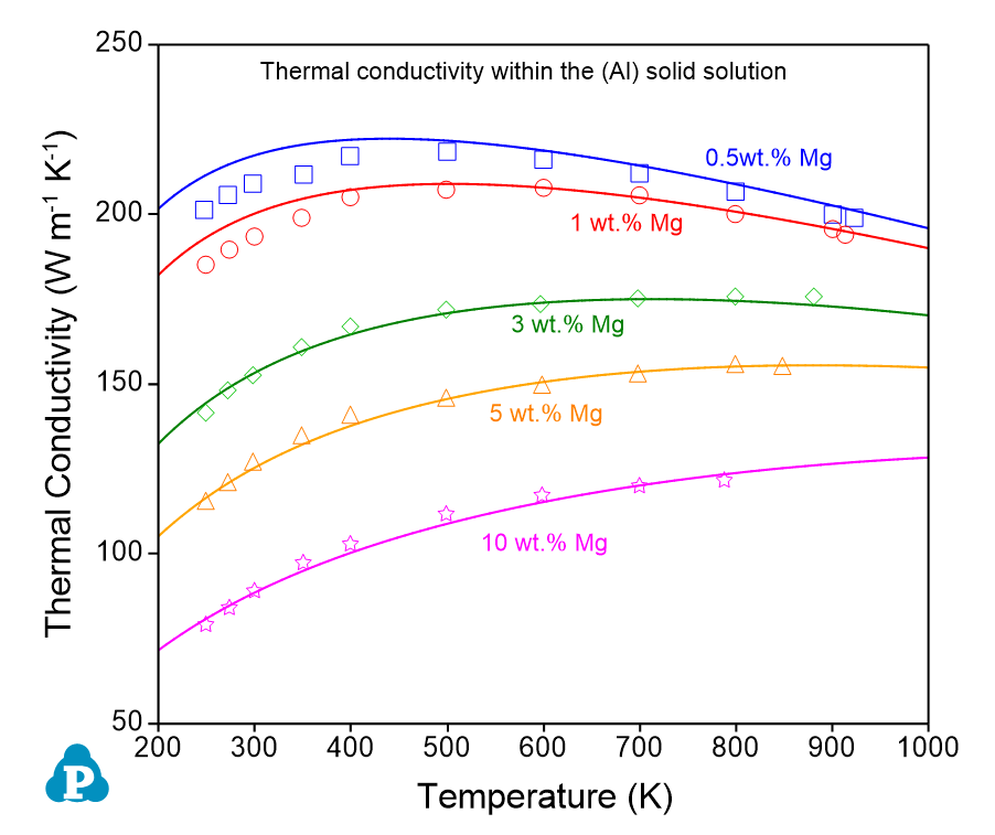
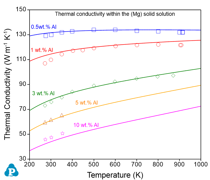
The comparisons between the calculated and measured thermal conductivities of the Al-Mg alloys are shown in Figure 9.9 . This example demonstrates the power and flexibility of the User-Defined Property function, which allows users to define a wide range of material properties. The property must be expressed as a function of phase compositions or site fractions that can be calculated by PanPhaseDiagram module.
|
(a) |
(b) |
|
Figure 9.9: Comparison between the calculated and measured thermal conductivities in (a) the (Al) solid solution and (b) the (Mg) solid solution, in the Al-Mg binary system |
|
[1991Hel] J. Helsing, G. Grimvall, Thermal Conductivity of Cast Iron: Models and Analysis of Experiments. J. Appl. Phys. 70 (1991) 1198–1206.