Simulation of Hardness of Aluminum Alloy 6005

Example 3.4: Simulation of Hardness of Aluminum Alloy 6005

Purpose: Learn to calculate the particle size, number density and hardness of aluminum alloy 6005
Module: PanEvolution
Thermodynamic and Mobility Database: Al_Demo.rtdb
Kinetic Parameters Database: Al_Alloy.kdb
Batch file: Example_#3.4.pbfx

Calculation Procedures:

Create a workspace and select the PanEvolution module following Pandat User’s Guide: Workspace;
Load Al_Demo.rtdb following the procedure in Pandat User’s Guide: Load Database, and select Al, Mg, Si three components;
Click on PanEvolution/PanPrecipitation on the menu bar and select "Load KDB or EKDB", then select the Al_Alloy.kdb; the pop-out window is shown in Figure 3.4.1 which include the alloy name, the matrix phase and the precipitate phase, and select the AA6xxx alloy in the "Define Alloy Parameters" column;
Open the Al_Alloy.kdb from workspace through the menu "File → Open File", and view the kinetic parameters;
Click on the menu "PanEvolution/PanPrecipitation → Precipitation Simulation", and set up the calculation condition as shown in Figure 3.4.2. Note the alloy composition is wt% (click Option button to select the unit);

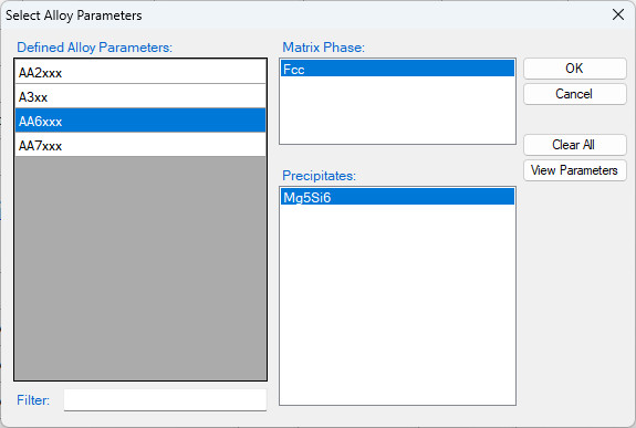
Figure 3.4.1: The matrix phase and the precipitate phase for AA6005

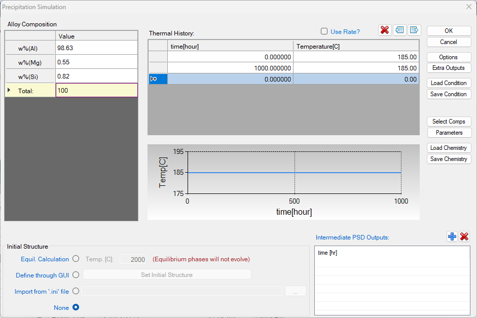
Figure 3.4.2: Setup alloy composition and heat treatment condition as ageing at 185°C for 1000 hours

Post Calculation Operation:

The default plot shows the total volume fraction of the Mg5Si6 phase as a function of time shown in Figure 3.4.3.
Create a new table as shown in Figure 3.4.4, and plot the log10(time) vs. log(nd), log10(time) vs. log(size), and log10(time) vs. hv;
Right Click on the Table node below the Graph and choose "Import Table from File", import three tables: AA6005-nd_exp.dat, AA6005-size_exp.dat, and AA6005-hv_exp.dat one by one;
Plot the experimental data in the corresponding plot by drag in the x-axis and then press Ctrl and drag in the y-axis of the experimental data table;
The default plot of the experimental data is a line instead of points. In the Property Window, change the Plot Type as Point;
Change graph appearance following the procedure in Pandat User’s Guide: Property;
Add legend for graph following the procedure in Pandat User’s Guide: Icons for Graph on Toolbar;

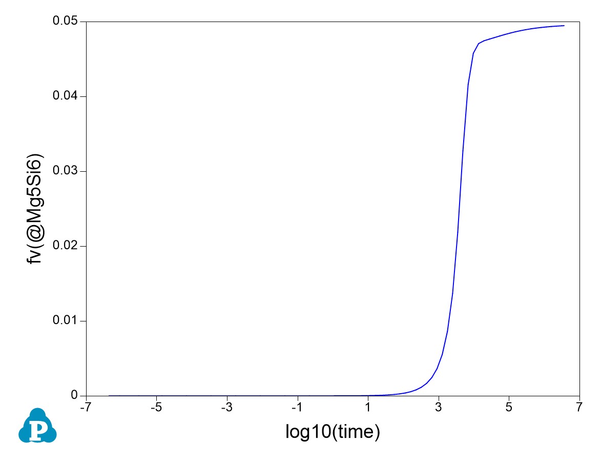
Figure 3.4.3: Default plot of volume fraction evolution of the precipitate

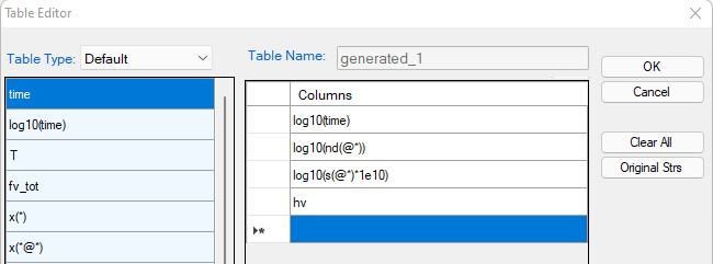
Figure 3.4.4: Create a new table

Information obtained from this calculation:

Figure 3.4.3 shows the default plot of the simulation which is volume fraction evolution of the precipitate phase. The time is in second;
Figure 3.4.5 shows the calculated number density evolution; Figure 3.4.6 shows the size evolution, and Figure 3.4.7 the hardness change with time. Experimental data are plotted on them for comparison;
It is seen that the number density reaches the highest value at ~1000 s (~0.3 h), but the particle size is very small. The hardness reaches peak at ~10000 s (~2.8 h) when both the number density and the particle size are favorable.

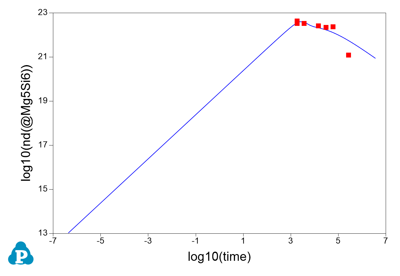
Figure 3.4.5: Calculated evolution of the particle number density with experimental data

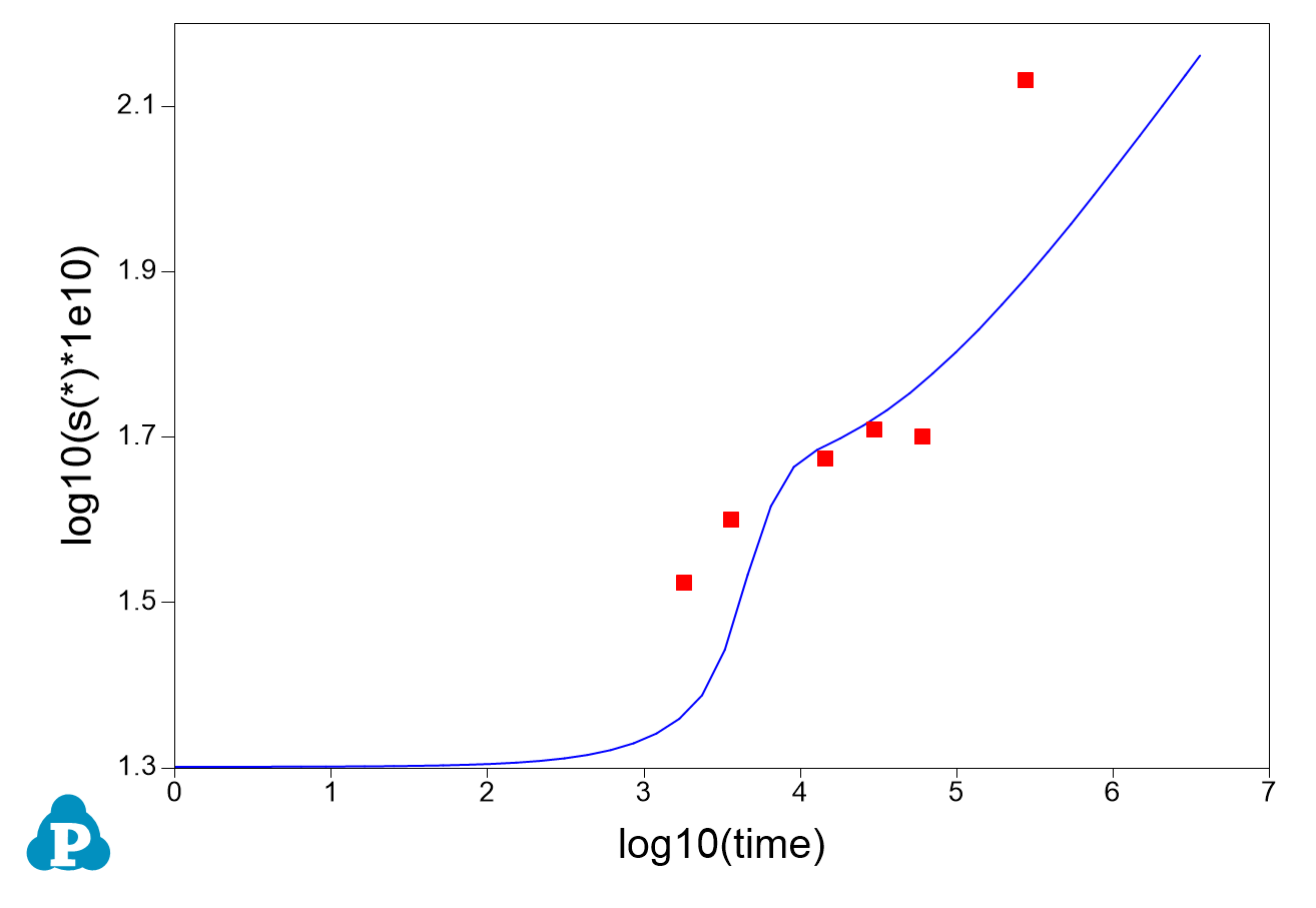
Figure 3.4.6: Calculated evolution of the particle size with experimental data

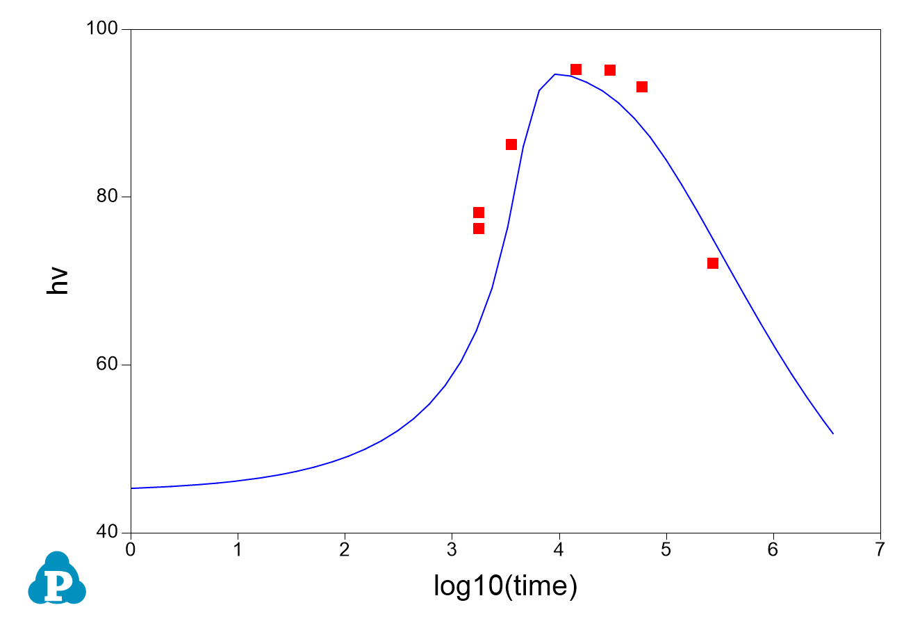
Figure 3.4.7: Calculated evolution of hardness with experimental data