Example 4.6: Carburization with Fixed Composition at Boundary
Purpose: Learn to perform diffusion simulation at constant temperature for a carburization process with a fixed chemical composition at boundary.
Module: PanDiffusion
Thermodynamic and Mobility Database: Fe-Demo.rtdb
Batch file: Example_#4.6.pbfx
Calculation Procedures:
- Create a workspace and select the PanDiffusion module following Pandat User’s Guide: Workspace;
- Load Fe-Demo.rtdb following the procedure in Pandat User’s Guide: Load Database, and select Fe, Si, C three components;
- Click on the menu "PanDiffusion → Diffusion Simulation" and set up the calculation condition as shown in Figure 4.6.1. First click the red “X” above Regions to delete Region_2 and leave one Region only.
- Click on Region_1 and set the composition as 0.5C-99.5Fe (at%), the Diff. Length as 100 mm, and the # of Grids as 100.
- The Thermal History is set as 1200 K for 25 seconds;
- Click on Lower Boundary Condition (left edge of Region_1) and select “fixed_composition”, and set the Value as “x%(C)=3.0”;
- In the settings shown in Figure 4.6.1, composition profiles at the initial and final stages will be outputted. Click OK to perform calculations.
Post Calculation Operation:
- Enlarge the composition range between 0 and 4 (at%) to clearly display Carbon composition. The calculated plot is show in Figure 4.6.2 Change graph appearance and add text following the procedure in Pandat User’s Guide: Property.
Information obtained from this calculation:
- Carbonization process in Fcc phase in the Fe-C system. Lower boundary condition is a fixed carbon composition;
- After holding the material at 1200K for 25 seconds, composition profiles can be viewed at final stage (25 s). The carbon gradually diffused into the Fcc phase from the boundary;
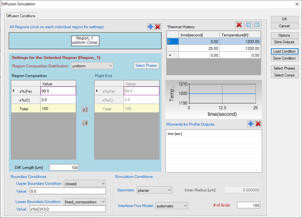
Figure 4.6.1: Setting of the simulation condition
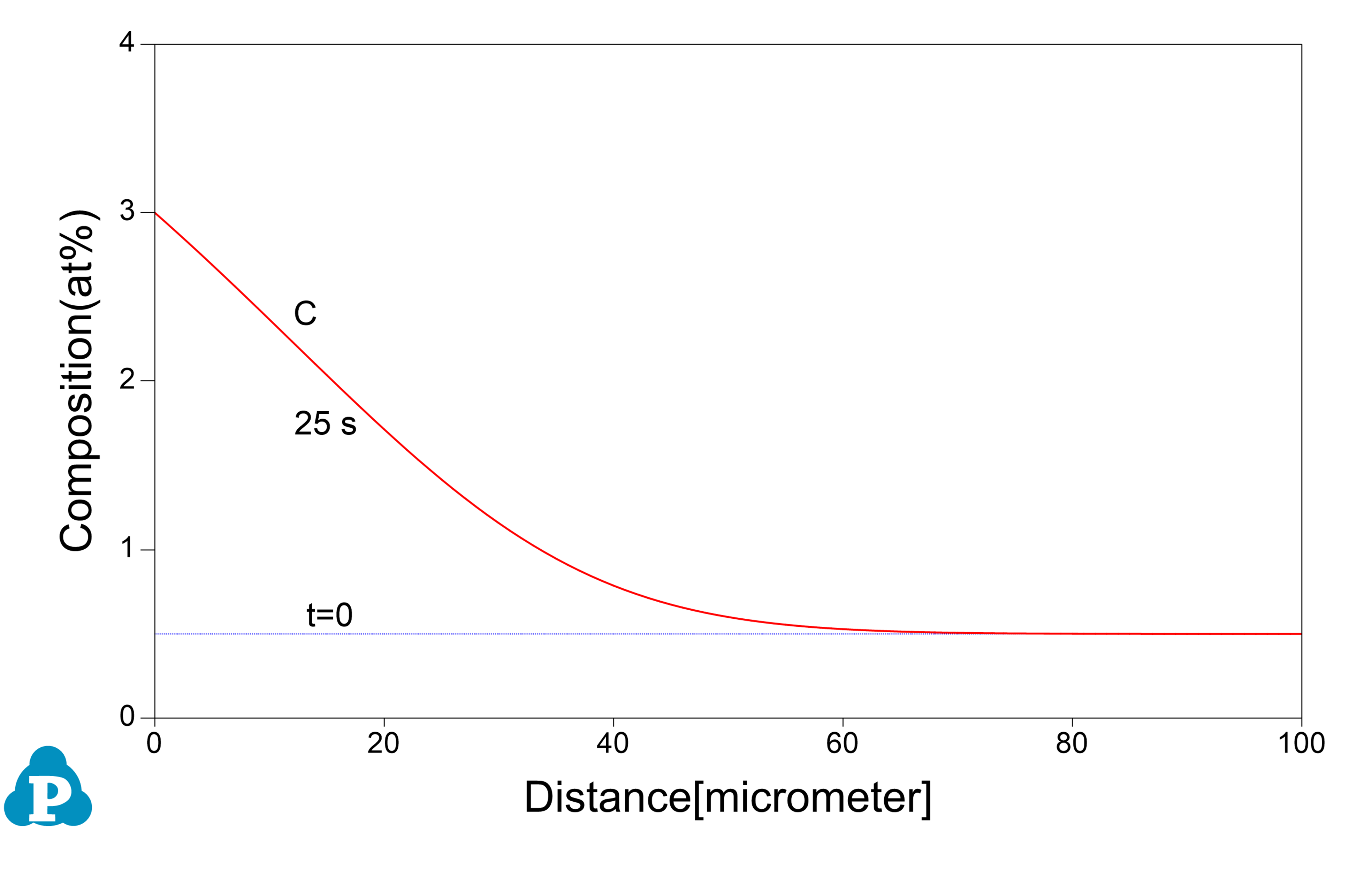
Figure 4.6.2: Calculated C composition profile for diffusion at 1200K for 25s