Example 4.11: Fe-Si-C Uphill Diffusion
Learn to perform uphill diffusion simulation in a Fcc matrix at a constant temperature.
Purpose: Learn to perform uphill diffusion simulation in a Fcc matrix at a constant temperature.
Module: PanDiffusion
Thermodynamic and Mobility Database: Fe-Demo.rtdb
Batch file: Example_#4.11.pbfx
Calculation Procedures:
- Create a workspace and select the PanDiffusion module following Pandat User’s Guide: Workspace;
- Load Fe-Demo.rtdb following the procedure in Pandat User’s Guide: Load Database and select Fe, Si, C three elements;
- Click on the menu "PanDiffusion → Diffusion Simulation" or click the icon
 and set up the calculation condition as shown in Figure 4.11.1;
 - Click on “Select Phases” and make Fcc the entered phase, while other phases are suspended;
- Click on Region_1 and set the composition as Fe-3.8Si-0.49C (wt%). In Region_1, set the length (Diff. Length) as 25 mm.
- Click on Region_2 and set the composition as Fe-0.05Si-0.45C (wt%). In Region_2, set the length (Diff. Length) as 25 mm;
- The Thermal History is a period of 312 hours (13 days) with a constant temperature at 1050 °C;
- The total number of grids (# of Grids) is 100;
- In the settings shown in Figure 4.11.1, composition profiles at the initial and final stages, as well as 100 and 200 hours, will be outputted. Click OK to perform calculations;
- Details on these options can be found in Pandat User’s Guide: Settings in General Diffusion Simulation.
Post Calculation Operation:
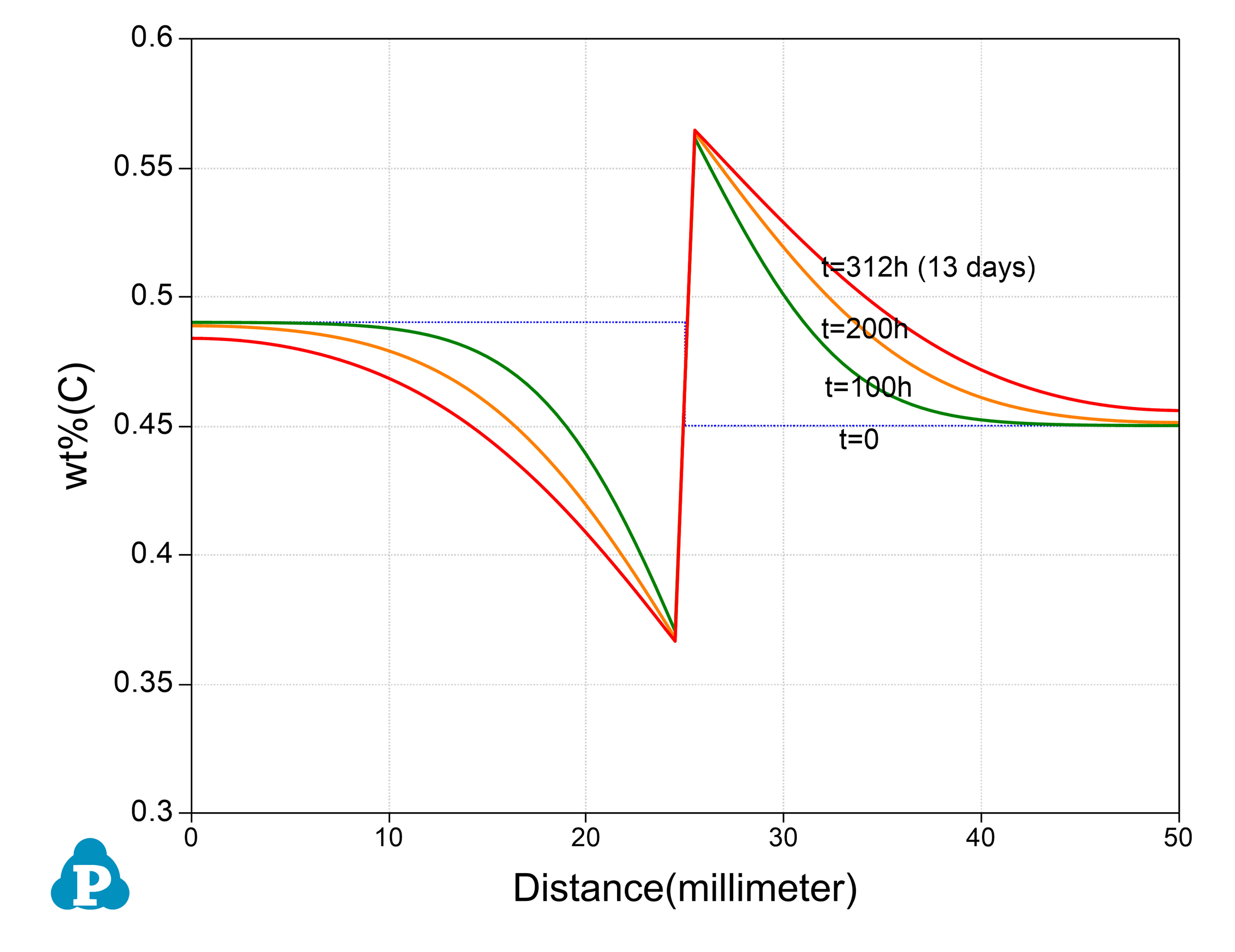
- Set the scale of the Y axis to be 0.3-0.6 (wt%); Remove composition profiles of Fe and Si; Add grid to the graph by setting “Show Major Grid” as "True" in the property window; The calculated plot is show in Figure 4.11.2.Change graph appearance and add text following the procedure in Pandat User’s Guide: Property.
Information obtained from this calculation:
- Composition profile of carbon in Fcc Matrix after an uphill diffusion.
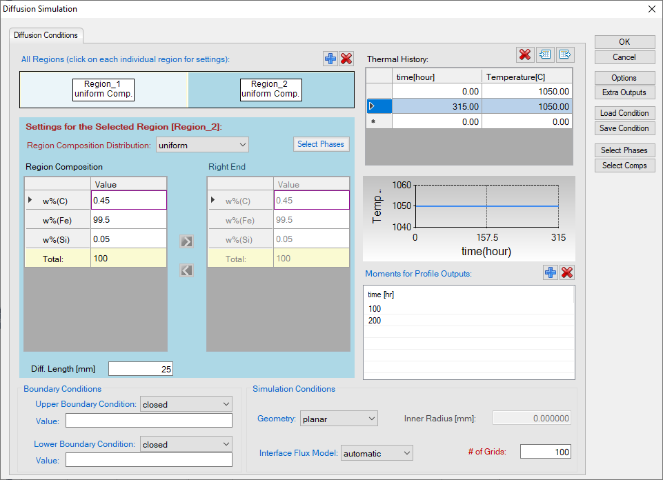
Figure 4.11.1: Setting of the simulation condition