Calculation of Martensite Start Temperature in a 2D Isopleth

Example 1.31: Calculation of Martensite Start Temperature in a 2D Isopleth

Purpose: Learn to calculate the starting temperature of martensite in a 2D isopleth
Module: PanPhaseDiagram
Database: Fe_Demo.rtdb
Batch files: Example_# 1.31.pbfx

Calculation Procedures:

Load Fe_Demo.rtdb database following the procedure in Pandat User’s Guide: Load Database, and select Fe, C, Cr three components.
From menu “PanPhaseDiagram → Martensite Start Temperature”, set the calculation conditions as shown in Figure 1.31.1. It is an isopleth section calculation with the Cr content fixed at 10 at.%, the C content varies from 0 to 2 at.%, and the temperature ranges from 400 to 1000 K.

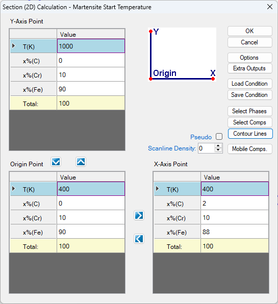
Figure 1.31.1: The conditions of the section calculation

Then click the Contour Lines button in Figure 1.31.1 to open the contour-line setting window, as shown in Figure 1.31.2. First, we need to define the Contour Type.
Note: Ms_Lath and Ms_Plate correspond to the Fcc → Bcc martensitic transformation with lath and plate morphology, respectively. Ms_Epsilon corresponds to the Fcc → Hcp martensite transformation, and Bs_G is used to calculate the Barnite start temperature. The setting shown in Figure 1.31.2 is for the calculation of Fcc → Bcc martensitic transformation with lath morphology. Since the martensite starting temperature is defined as the temperature at which the Gibbs energy difference between the Fcc phase and Bcc phase equals to zero, both the Start and Stop values of the contour line should be set to 0, with a step size of 1.

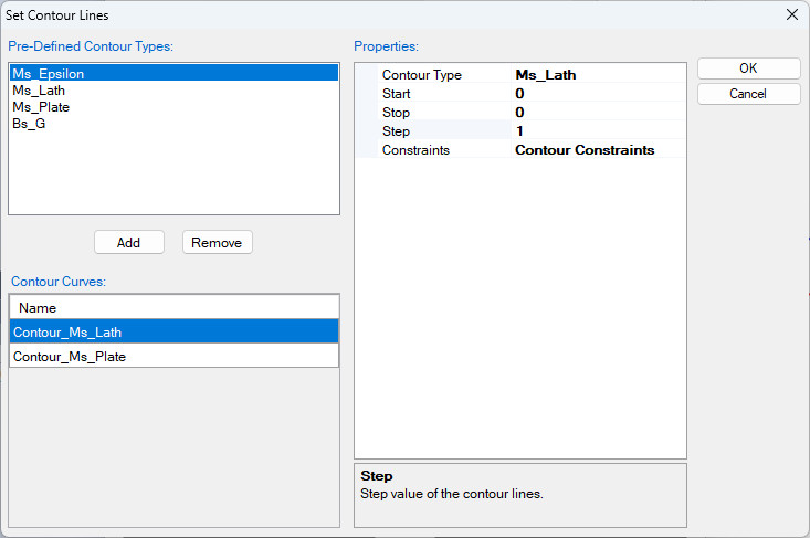
Figure 1.31.2: Set the contour line conditions for Ms_Lath and Ms_Plate.

Repeat the settings in Figure 1.31.1 and replace Ms_Lath with Ms_Plate in Figure 1.31.2, the martensite start temperature for the Fcc → Bcc martensitic transformation with plate morphology can be calculated.
The calculated martensite start temperatures temperatures for the Fcc → Bcc martensitic transformation with both lath and plate morphologies are calculated as shown in Figure 1.31.3 for the isopleth section defined in Figure 1.31.1. Experimental data are also plotted for comparison (refer Example 1.26 for more information on adding experimental data on a plot). The blue line and solid square represent the calculated and measured martensite transformation temperatures with lath morphology, while the red line and solid circle represent those with plate morphology.

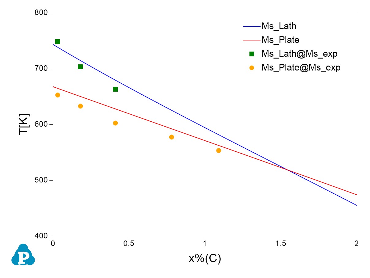
Figure 1.31.3: Calculated results of martensite start temperature Ms_Lath and Ms_Plate compared with experimental data.

More Information about this Example:

This example demonstrates how to calculate the starting temperature of Martensite transformation through Pandat GUI.
The calculation can also be performed through batch calculation. Example_#1.31.pbfx is provided in the folder. It should point out that when contour lines options is included in the section calculation, individual_phase must be set as “true” in the condition section of the batch file, as shown below:

Ms_Epsilon, which refers to Fcc to Hcp martensite transformation can also be calculated using similar procedures for Fe–Mn–based steels.