Calculate Open Circuit Voltage (OCV) under Equilibrium Condition

Purpose: Learn to perform equilibrium calculation, use extra output table and extra output graph to output chemical potential and voltage value to simulate the open circle voltage curve of an alloy system for battery application.
Module: PanPhaseDiagram
Database: LiSn.tdb
Background: Carbon based anode material is widely used in Li-ion batteries. But its low charge density motivates the search for next generation of anode materials. Sn based alloy is one of potential anode candidates. The calculation of open circle voltage curve of the Li-Sn system sheds a light on the potential capacity of the alloy system. This example shows how to calculate the open circle voltage curves directly from PanPhaseDigaram modular and compare with experimental data. In an alloy system, the equilibrium open-circle voltage E is associated with chemical potential through the Nernst equation: . F is Faraday’s constant, 94685 C/volt. In this example of Li-Sn system, n = 1, then . At 688 K, Li and Sn are in liquid state, so the reference state is liquid Li.

Calculation Method 1:

Create a workspace and select the PanPhaseDiagram module following Pandat User’s Guide 2.1;
From menu bar click Batch Calc-> Batch Run, select Example_#1.26.pbfx;

Calculation Method 2:

Create a workspace and select the PanPhaseDiagram module following Pandat User’s Guide 2.1;
Load tdb following the procedure in Pandat User’s Guide 3.2.1;
Start line calculations, click PanPhaseDiagram -> Line Calculations or click the icon from the toolbar.
A line calculation setting window will pop up as shown in Figure 1. The temperature is set as 688 K, as experimental data are available at 688 K for comparison. The composition range is from pure Sn, i.e. x(Sn) = 1, to pure Li, i.e. x(Li) = 1. The Number of steps is set to be 200

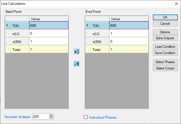
Figure 1. Line calculation conditions setting

Set “Extra Outputs table”. In order to output the open-circle voltage value, some extra outputs are required. Click “Extra Outputs” in the interface shown in Figure 1, a new interface will appear as shown in Figure 2. Then click the blue “+” symbol to pop out the Table Editor as shown in Figure 3. From this Table Editor, one can select to output Extra properties which are not shown in the default table.

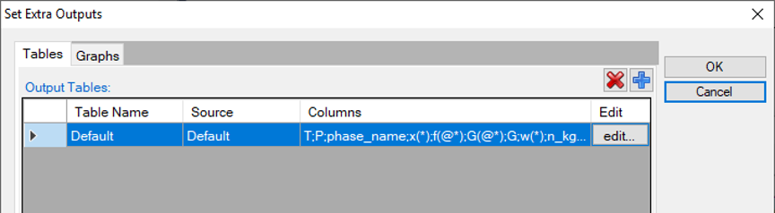
Figure 2. Interface to set Extra Output

In this example, we output mu(Li:Liquid[Li]) as the chemical potential of Li in the system with reference to the liquid phase, i.e. . Then, we add another quantity -mu(Li:Liquid[Li])/96485 which is equivalent to in this system. The quantity x(Li)/x(Sn) represents the y in Li_ySn system. The settings are shown in Figure 3. After setting the table editor, click OK.
Tips: The properties can be dragged from the left column to the right column, or directly type in the right column. When click a property in the left column, the description of this property is shown as description in the bottom of the interface. For example, in Figure 3, a(*:Liquid[*]); Description: Activity of component in system with given reference state. Some simple calculations are also applied in the table setting, such as -mu(Li:Liquid[Li])/96485 and x(Li)/x(Sn) in this example.

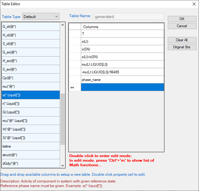
Figure 3. Define extra output table by drag properties from the left column to the right column or directly type in in the right column.

Set “Extra Outputs graph”. Click the icon “Graph” in “Set extra output” interface as shown in Figure 4, then click the blue “+” symbol to add extra Graph. An interface as shown in Figure 5 will appear. Select the “generated” table set in previous step in the “Table source”. Drag x(Li)/x(Sn) from the left column to X axis in the right column; drag -mu(Li:Liquid[Li])/96485 from the left column to Y axis in the right column. Then click OK.
When the interface goes back to Figure 1, click OK. Calculation starts.

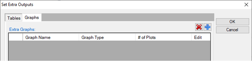
Figure 4. Set Extra Output Graphs interface

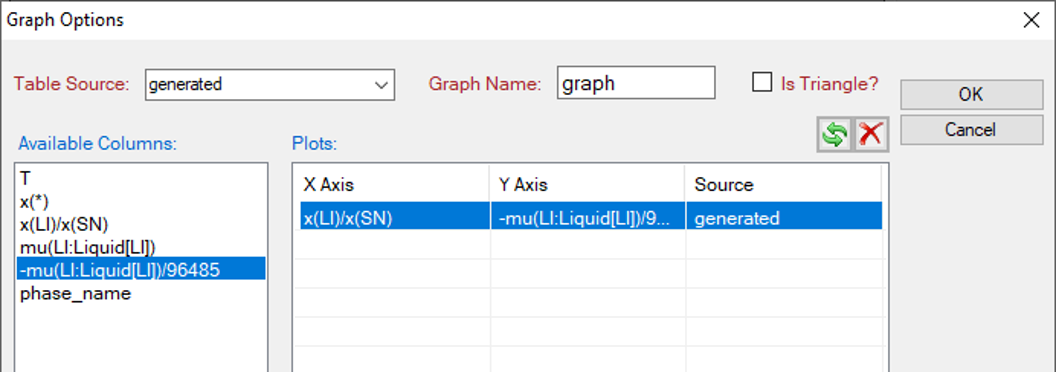
Figure 5. Output Graphs option interface

Post Calculation Operation:

Rescale the axis, and edit the axis title.
After the calculation, the calculated open circle voltage curve of Li-Sn system is shown in Figure 6 with the default settings. Set the x-axis range from 0 to 6, and obtained as shown in Figure 7

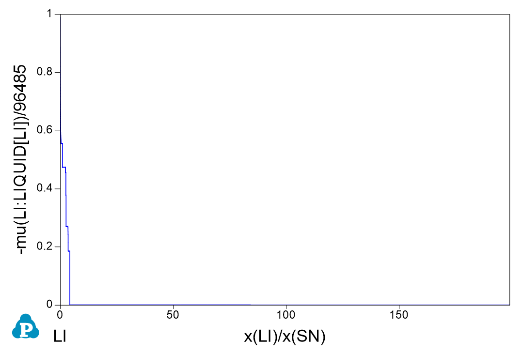
Figure 6. Calculated open circle voltage curve of Li-Sn system.

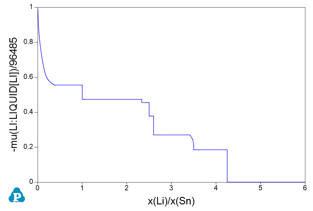
Figure 7. Calculated open circle voltage curve of Li-Sn system: Rescale x-axis of x(Li)/x(Sn) to 0-6.

Import experimental data. From the menu, click Table -> Import Table From Files, choose LiSn.txt file to import the experimental data table into the Pandat workspace.
Compare calculated results with experimental data. From the menu, click Graph -> Edit Plots, or click the button from the toolbar to open the setup Plot interface as shown in Figure 8. Select the imported LiSn table, choose LixSn as X axis, and E_Li(V) as Y axis. Then click OK.

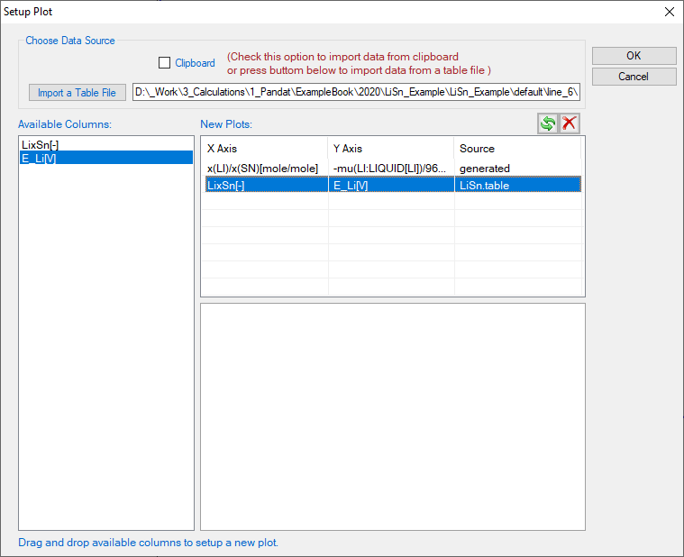
Figure 8. Setup Plot, add the experimental data into generated figure

Then change “Plot Type” as “Point”, “Marker Color” as “Transparent”, “Marker Style” as “Circle”; Then experimental data are changed to red open symbol, added legend, change the Title of Y axis as (E vs E_Li ) / V. The final produced figure is shown in Figure 9.

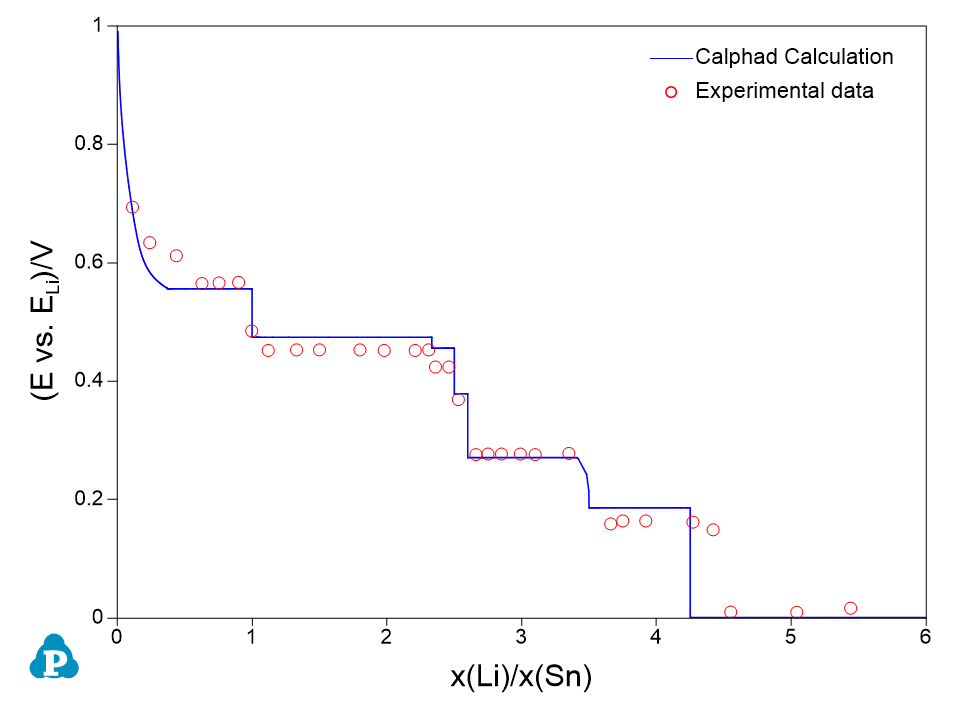
Figure 8. Setup Plot, add the experimental data into generated figure