Co-precipitation of γ’ and γ” in the Ni-Al-Nb Pseudo-ternary System
- Purpose: Learn to calculate co-precipitation of γ’ and γ” for an alloy in a pseudo-ternary system;
- Module: PanEvolution/PanPrecipitation
- Database: NiAlNb_Pseudo.tdb and Ni-2.4Al-3.8Nb.kdb
Calculation Method 1:
- From menu bar click Batch Calc-> Batch Run, select Example_#3.3.pbfx;
Calculation Method 2:
- Create a workspace and select the PanPrecipitation module following Pandat User’s Guide 2.1;
- Load NiAlNb_Pseudo.tdb following the procedure in Pandat User’s Guide 3.2.1;
- Click on PanEvolution/PanPrecipitation on the menu bar and select Load KDB, then select the Ni-2.4Al-3.8Nb.kdb, the pop-out window is shown in Figure 1 which include the alloy name, the matrix phase and the precipitates. Two precipitates are defined in this case;
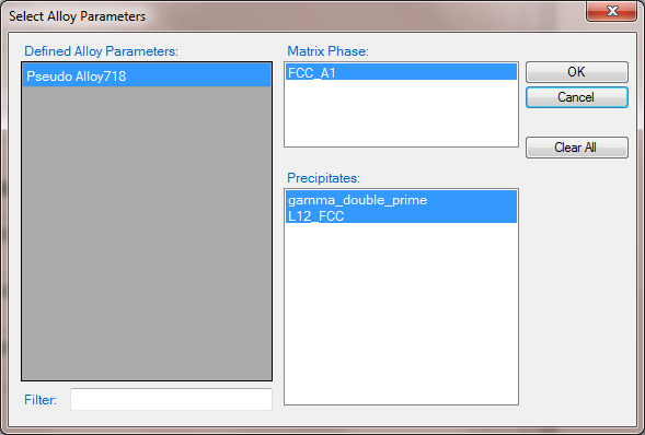
Figure 1. Pop-out window when loading the Ni-2.4Al-3.8Nb.kdb
- Open the Ni-2.4Al-3.8Nb.kdb from Pandat workspace through File->Open File, and view the kinetic parameters as shown in Figure 2;
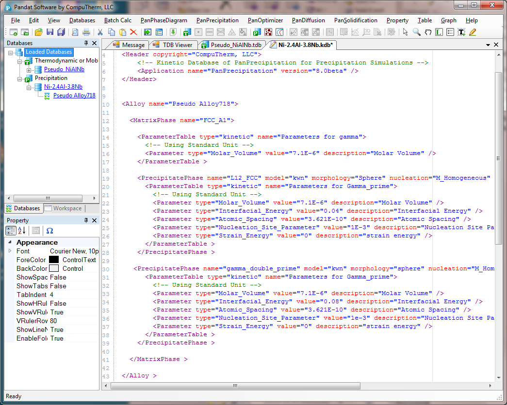
Figure 2. Open the Ni-2.4Al-3.8Nb.kdb in Pandat workspace to view the kinetic parameters of the two precipitate phases
- Click on PanEvolution/PanPrecipitation->Precipitation Simulation, and set up the calculation condition as shown in Figure 3;
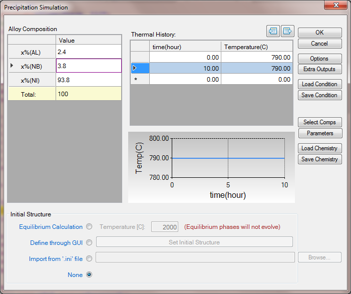
Figure 3. Precipitation simulation of alloy Ni-2.4Al-3.8Nb ageing at 790oC for 10h
Post Calculation Operation:
- The default plot shows the total volume fraction of and γ” as a function of time;
- Open the Default Table, create time vs. volume fractions of γ’ and γ”, and time vs. sizes of g¢ and g¢¢ plots as shown in Figure 4 and Figure 5;
- Change graph appearance following the procedure in Pandat User’s Guide 2.3.1;
- Add legend following the procedure in Pandat User’s Guide 2.3.3;
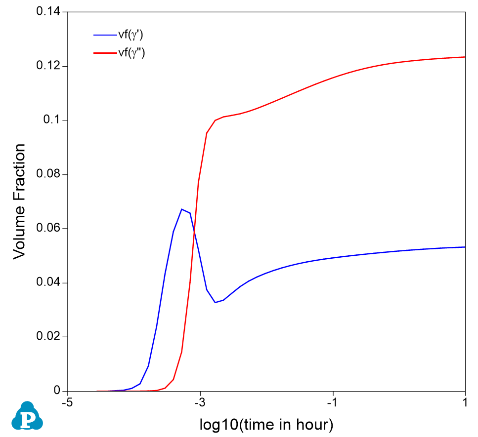
Figure 4. Calculated volume fraction evolution of the two precipitate phases
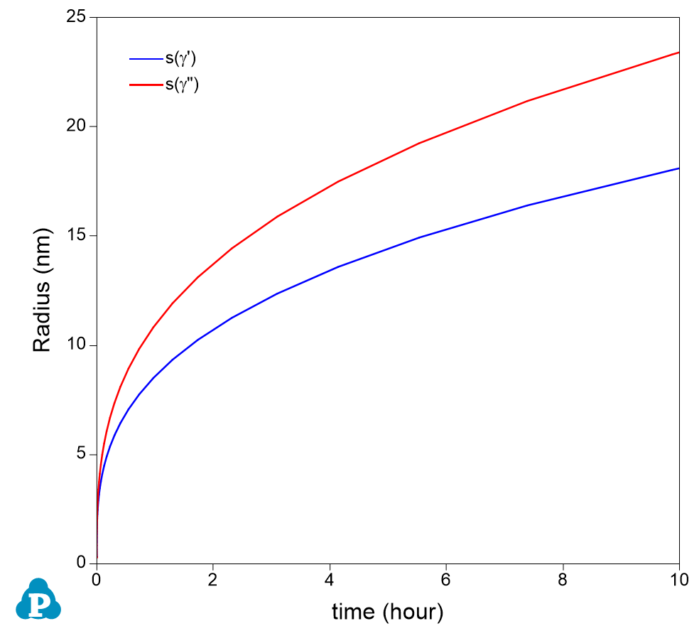
Figure 5. Calculated average size evolution of the two precipitate phases
Information obtained from this calculation:
- Figure 4 shows the calculated evolution of volume fraction of the two precipitate phases. It is seen that γ’ precipitated quickly at very early stage, but gave way to γ” at later time;
- Figure 5 shows the calculated evolution of the average size of the two precipitate phases. It is seen that γ” is bigger than γ’;
- Add a new table as shown in Figure 6 with the Table Type as psd. The Columns are particle sizes and number densities with (@*) means all precipitate phases. The default calculated size is in meter, which is converted to nm by multiplying the column by 1e+9. The default calculated number density is number/m^3, which is converted to mol/m^3. The index=i means to populate the size and number density at the final state t=10h;
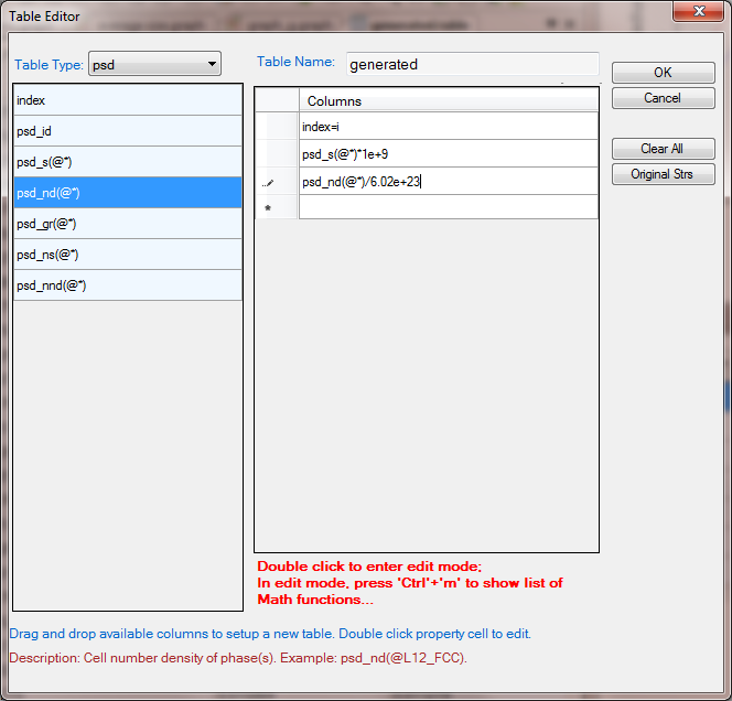
Figure 5. Create a new table with particle sizes and number densities at final stage
- Plot particle size distribution from the new table by selecting the particle size as x-axis and number density as y-axis. Plot it for L12 (γ’) phase first and then add the one for γ” as shown in Figure 7;
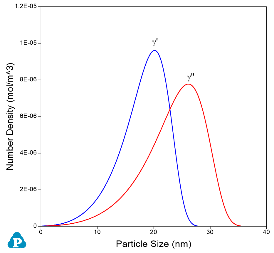
Figure 7. Particle size distributions of γ’ and γ” at final stage