Decarburization of Fe-C Matrix
- Purpose: Learn to perform diffusion simulation at constant temperature for a carburization process with a fixed chemical composition at boundary
- Module: PanDiffusion
- Database: Fe-Si-C.tdb
Calculation Method 1:
- From menu bar click “Batch Calc-> Batch Run”, select Example_#4.14.pbfx;
Calculation Method 2:
- Create a workspace and select the PanDiffusion module following Pandat User’s Guide 2.1;
- Load Fe-Si-C.tdb, and select component Fe and C, following the procedure in Pandat User’s Guide 3.2.1;
- Click on “PanDiffusion->Diffusion Simulation” or click the icon
 to open a setting dialog and select the proper units
 - Firstly, click
 of “All Regions” to delete Region_2;
 - Click on Region_1 and set a uniform composition distribution of Fe-0.5C (at%); The length ( Length) of Region_1 is 100 um;
- The total number of grids (# of Grids) is 100;
- The Thermal History is a period of 10 seconds with a constant temperature at 1000 oC;
- The Lower Boundary Condition (left edge of Region_1) is a fixed “activity” of “a(C:graphite[*])=0.01”;
- The default output includes profiles of the initial and final compositions. To record a composition profile at a moment, click
 next to the “Moments for Profile Outputs” and input a time value. As shown in Figure 14.1, profiles at 1 second and 5 second will be outputted. Click OK to start calculation;
 - Details on these options can be found in Pandat User’s Guide sections 6.6.11 and 6.6.12.
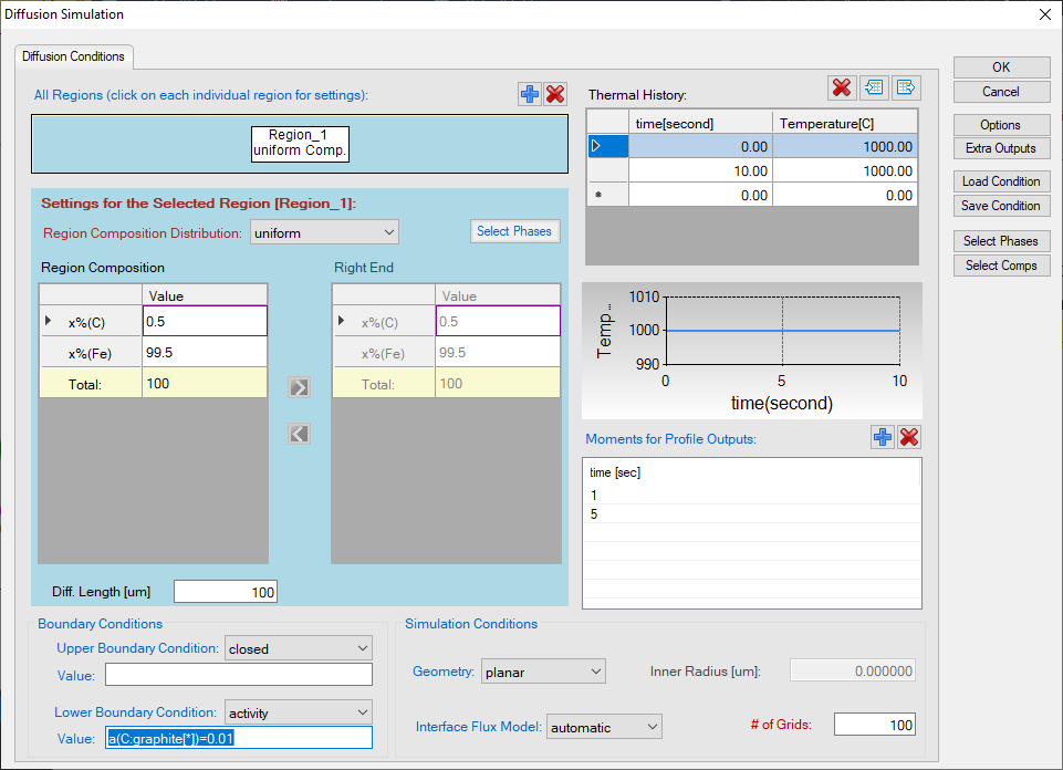
Figure 1. Settings applied in this example
Post Calculation Operation:
- Set the scale of the Y axis to be 0.1-0.6 (at%). Remove composition profile of Fe. The calculated composition profiles are displayed in Figure 2. Add text and change graph appearance following the procedure in Pandat User’s Guide 2.3.1;
- Add grid to the graph by setting “Show Major Grid” to be True.
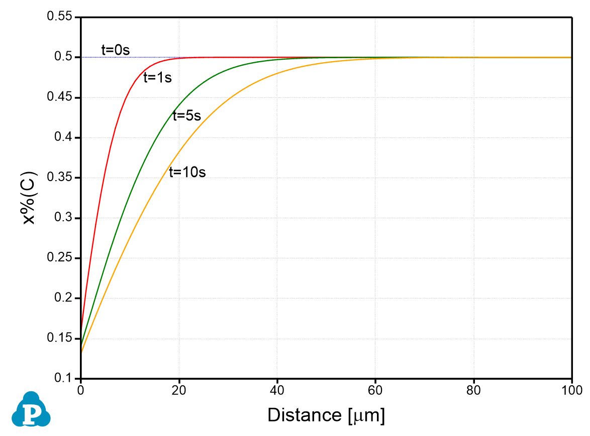
Figure 2. Simulation result of carbon composition profile
Information obtained from this calculation:
- Decarburization process in Fcc phase in the Fe-C system. Lower boundary condition is a fixed carbon activity (0.01, Graphite as the reference state)