Dissolution of a Single θ-Al2Cu Particle in FCC Matrix
- Purpose: Learn to perform single-particle dissolution simulation;
- Module: PanDiffusion
- Database: AlCu_MB.tdb
Calculation Method 1:
- From menu bar click “Batch Calc-> Batch Run”, select Example_#4.12.pbfx;
Calculation Method 2:
- Create a workspace and select the PanDiffusion module following Pandat User’s Guide 2.1;
- Load tdb, and select component Al and Cu, following the procedure in Pandat User’s Guide 3.2.1;
- Click on “PanDiffusion->Dissolution Simulation” or click the icon
 to open a setting dialog and select the proper unit of the simulation in the “Options”;
 - Click on “Select Phases” and make Fcc and AlCu_Theta the entered phases, while other phases are suspended;
- In Alloy Composition set a composition of Al-1.55Cu (at%);
- The total number of grids (# of Grids) is 100;
- The Geometry of particles is set to “Spherical”;
- In “Phase Information”, select Fcc as “Matrix Phase”.
- To add a particle, click
 bottom, then select AlCu_Theta in “Phase Name”. “Particle Size” is set to 0 um. “Vol. Fraction” is set to 0.008;
 - The “Thermal History” is a period of 35 minutes at 550oC;
- Click OK to start calculation;
- By default, dissolution simulation gives time-evolution of particle size as output. In order to display composition profile at desired moments, click next to the “Moments for Profile Outputs” and input a time value. As shown in Figure 12.1, profiles at 10 minutes and 15 minutes will be outputted. Click OK to start calculation;
- Details on these options can be found in Pandat User’s Guide sections 6.6.11 and 6.6.12.
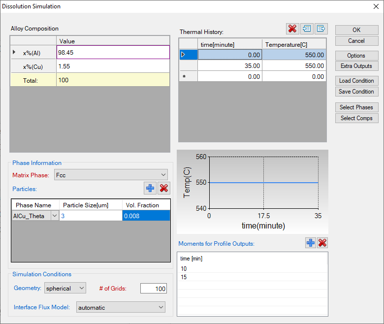
Figure 1. Settings applied in this example
Post Calculation Operation:
- The calculated particle dissolution with time is shown in Figure 2. User can modify it by changing the title, the scale and so on from the Property Window. User can also add experimental data by clicking Table -> Import Table From Files, and select Example_#4.12.txt, and then follow Example 3.1 to add the experimental data on the plot. More information can be found in Pandat User’s Guide 2.3.1.
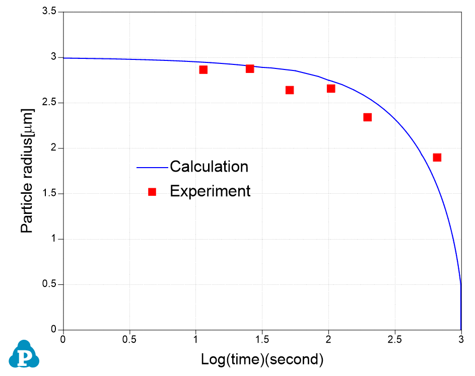
Figure 2. The simulation result of particle-size evolution
- Click and open the Default table and select “distance”, “x%(Al)” and “x%(Cu)” to plot the composition profiles at starting, ending and the two selected intermediate times as shown in Figure 3.
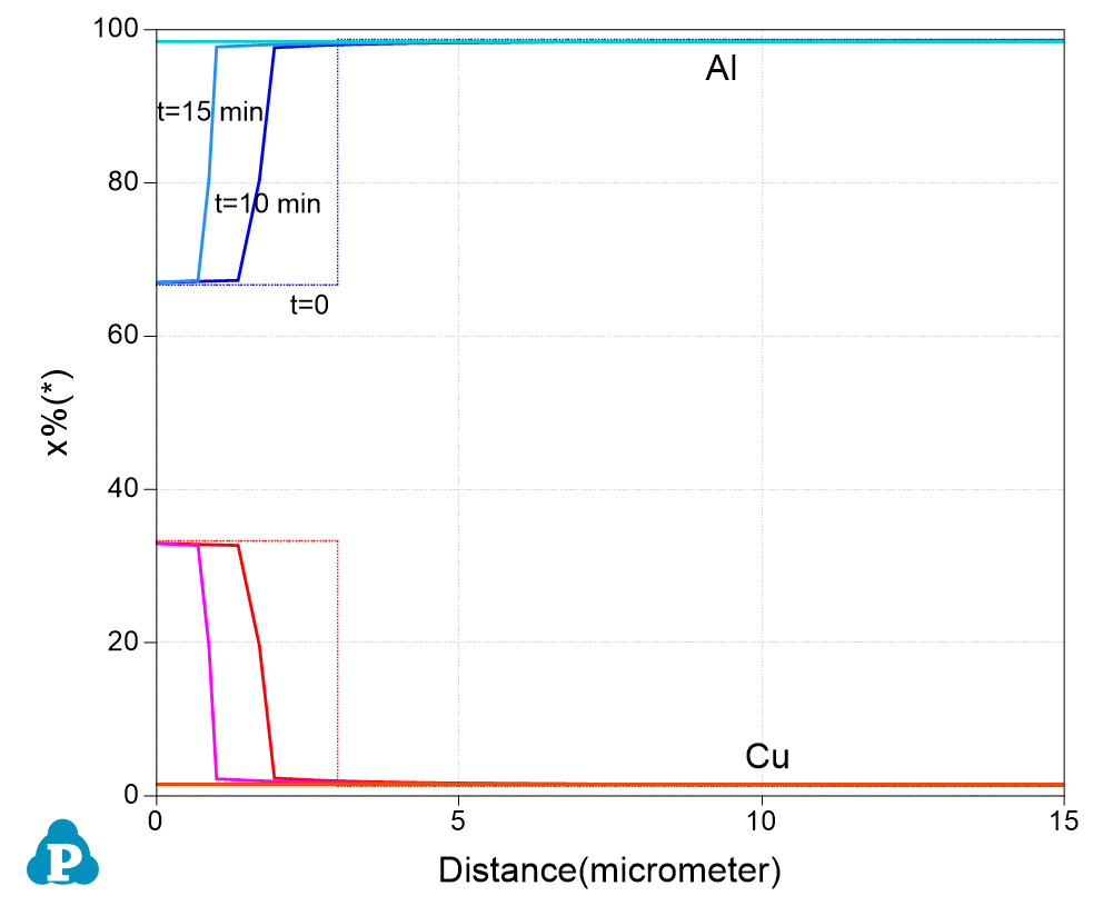
Figure 3. The simulation result of composition-profile evolution