Simulation of Yield Strength of Aluminum Alloy 357
- Purpose: Learn to calculate yield strength including intrinsic, solid solution, and precipitation strengthening of aluminum alloy 356 during the process of ageing.
- Module: PanEvolution/PanPrecipitation
- Database: AlMgSi.tdb and AA3xx.kdb
Calculation Method 1:
- From menu bar click Batch Calc-> Batch Run, select Example_#3.6.pbfx;
Calculation Method 2:
- Create a workspace and select the PanPrecipitation module following Pandat User’s Guide 2.1;
- Load AlMgSi.tdb following the procedure in Pandat User’s Guide 3.2.1;
- Click on PanEvolution/PanPrecipitation on the menu bar and select Load KDB, then select the AA3xx.kdb;
- Click on PanEvolution/PanPrecipitation->Precipitation Simulation, and set up the calculation condition as shown in Figure 1. Note that the “Equilibrium Calculation” button under Initial Structure (bottom) should be checked and the solution temperature (540oC in this case) should be given;
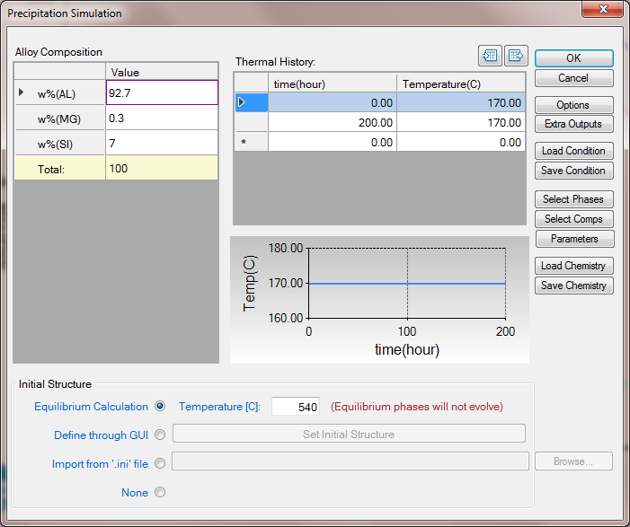
Figure 1. Setup calculation condition for aluminum alloy 356
Post Calculation Operation:
- Change graph appearance following the procedure in Pandat User’s Guide 2.3.1;
- Add legend following the procedure in Pandat User’s Guide 2.3.3;
- Create a new table as shown in Figure 2, and select all the columns in the newly created table to create a plot;
- Click Table below the Graph and choose Input Table from File, input table: AA356-ys_exp.txt; Note that the extension of a data file can be either txt or dat;
- Plot the experimental data in the corresponding plot by drag in the x-axis and then press Ctrl and drag in the y-axis of the experimental data table;
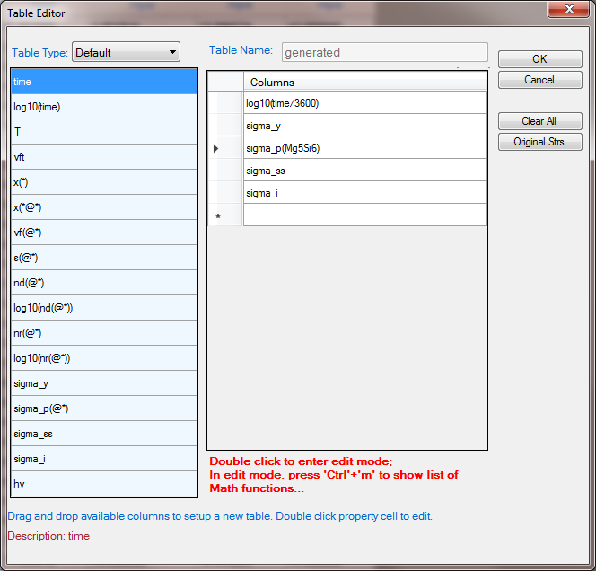
Figure 2. Create a new table for yield strength plot
Information obtained from this calculation:
- Figure 3 shows a comparison of the calculated yield strength (lines) with the experimental data (symbols). The green line (symbol) represents the intrinsic contribution; the black line (symbol) represents the solid solution strengthening; the red line (symbol) represents the precipitation strengthening; and the blue line (symbol) is the total from all three contributions;
- Create a new table as shown in Figure 4, select log10(time/3600) as x-axis, and x%(Mg@_Fcc) and x%(Si@_Fcc) as y-axis to create a plot as shown in Figure 5;
- It is clearly seen from Figure 3 and Figure 5 that with the formation of Mg5Si6 precipitate, the solubility of Mg and Si in Fcc decreases and solution strengthening also decreases;
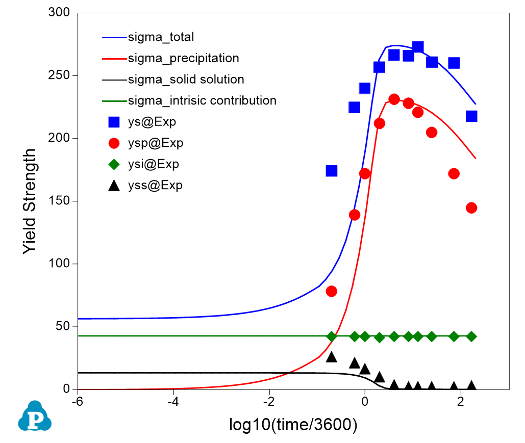
Figure 3. A comparison of the calculated yield strength (lines) with the experimental data (symbols)
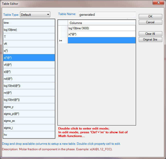
Figure 4. Create a new table to show the evolution of phase compositions
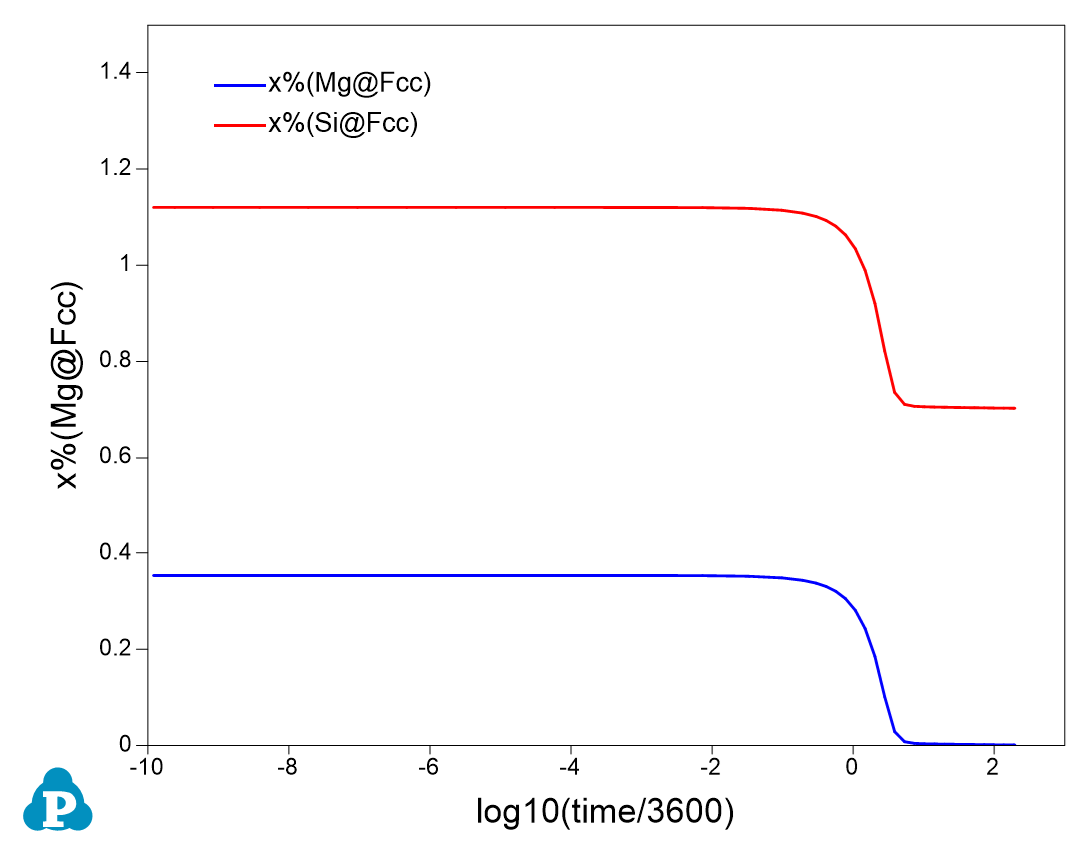
Figure 5. Evolution of elemental solubility in the matrix Fcc