Two-step aging of a binary Ni-Al alloy

Purpose: Learn to perform phase-field simulation of precipitation in a Ni-Al binary alloy under specified thermal conditions using PanPhaseField Module. Learn to use the features in PanPhaseField Module.
Module: PanPhaseField
Database: AlNi_Prep.tdb and AlNi.pfdb

Calculation Method 1

Create a workspace and select the PanPhaseField module following Pandat User’s Guide 2.1;
From menu bar click Batch Calc-> Batch Run, or click icon , then select Example_#6.1.pbfx;

Calculation Method 2:

Create a workspace and select the PanPhaseField module following Pandat User’s Guide 2.1;
Load TDB file AlNi_Prep.tdb through menu Database->Load TDB or PDB or by click icon , and select the elements: Al, Ni.
Load PFDB file AlNi.pfdb through menu PanPhaseField->Load PFDB or by click icon , select the available alloys: Mg alloys, as shown in Figure 1.
Set phase-field precipitation simulation conditions as shown in Figure 2. The alloy composition is Ni-15x.% Al. The first thermal stage is 850°C for 120 seconds. Then the temperature is reduced to 750 °C in 1 second. The second thermal stage is 750°C for another 120 seconds. Please pay attention to the units of the time and temperature when set conditions.
This 2D simulation uses a mesh grid of 128*128, and a length scale of 5E-9 m is applied. Please pay attention to the units of length when set conditions.
15 profiles of mesh grid will be outputted during the simulation.
Set number of threads to 8. If your computer has less than 8 threads, Pandat will automatically apply the max available threads on your computer.

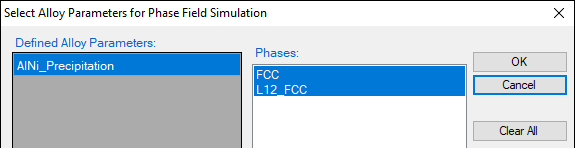
Figure 1. Loading the AlNi.pfdb file

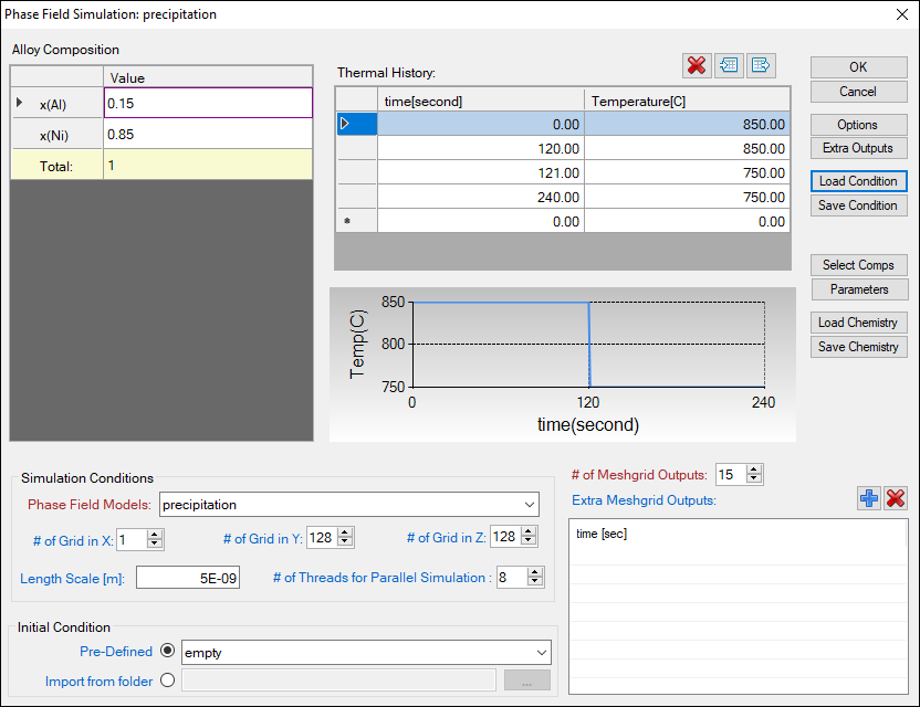
Figure 2. Set phase-field precipitation simulation conditions

Post Calculation Operation:

The default plot presents the time-evolution of phase volume fraction as shown in Figure 3, and the last frame of microstructure as shown in Figure 4.
Change graph appearance following the procedure in Pandat User’s Guide 2.3.1;
Add legend following the procedure in Pandat User’s Guide 2.3.3;
Add a new table as shown in Figure 5 with the Table Type as Default. Add columns of “time”, “dgm(@*)” as driving force of phases and “nr(@*)” as nucleation rate of phases.

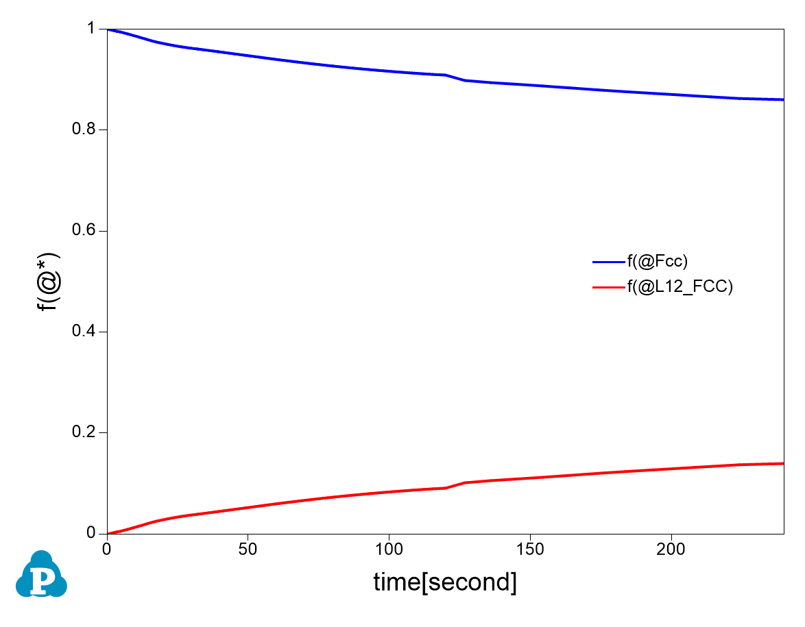
Figure 3. Default plot showing time-evolution of phase volume fraction

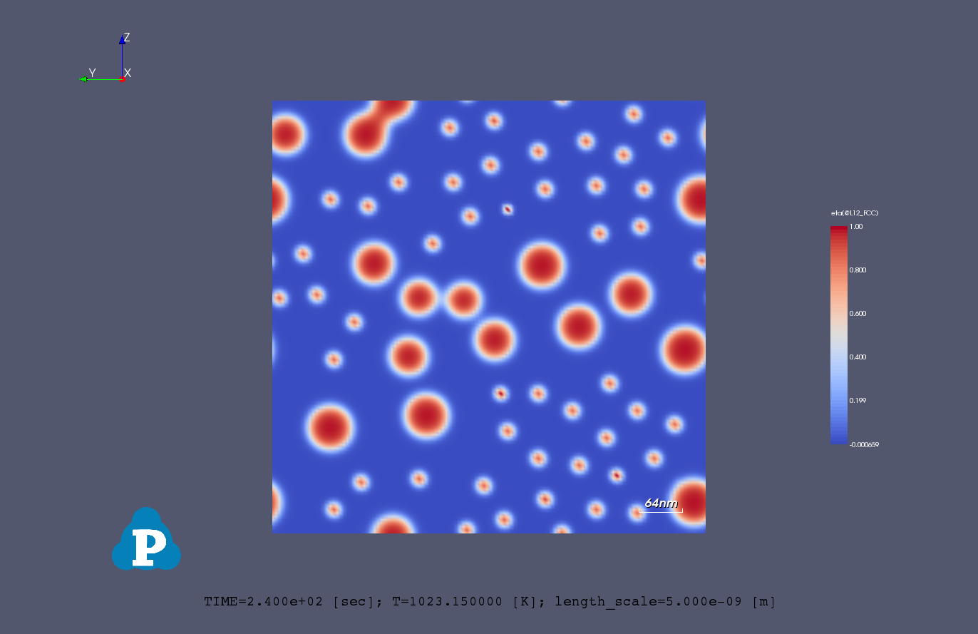
Figure 4. Default plot showing the last frame of L12 particle microstructure

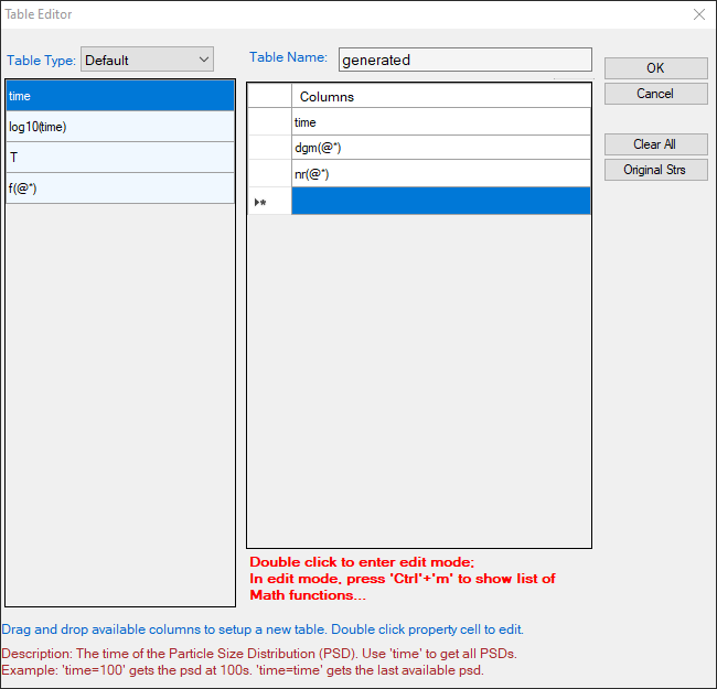
Figure 4. Create a new table with driving force and nucleation of phases

Plot driving force of L12 phase from the new table by selecting the time as x-axis and driving force dgm(@L12_FCC) as y-axis. The plot is shown in Figure 6.
Plot nucleation rate of L12 phase from the new table by selecting the time as x-axis and nucleation rate nr(@L12_FCC) as y-axis. The plot is shown in Figure 7.

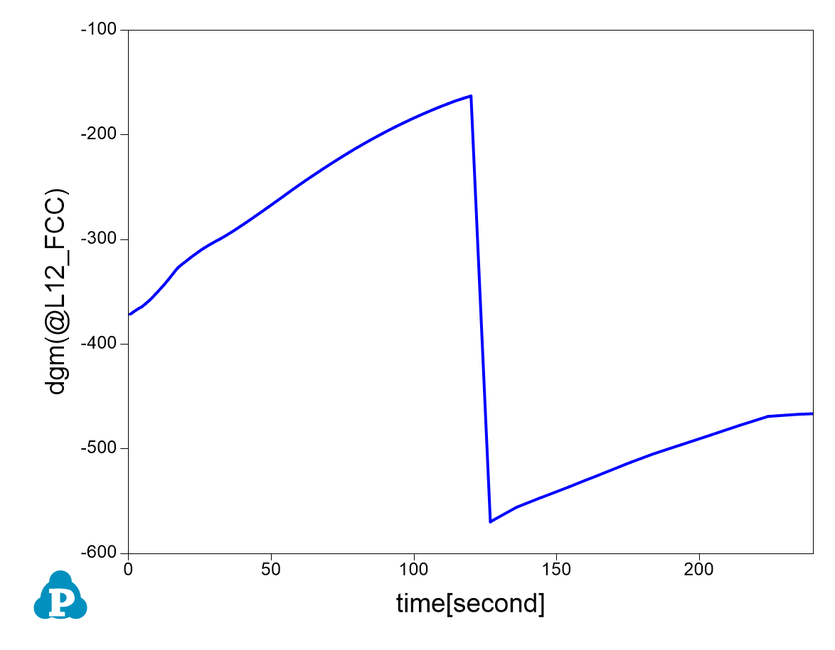
Figure 6. Time-evolution of driving force of L12 phase

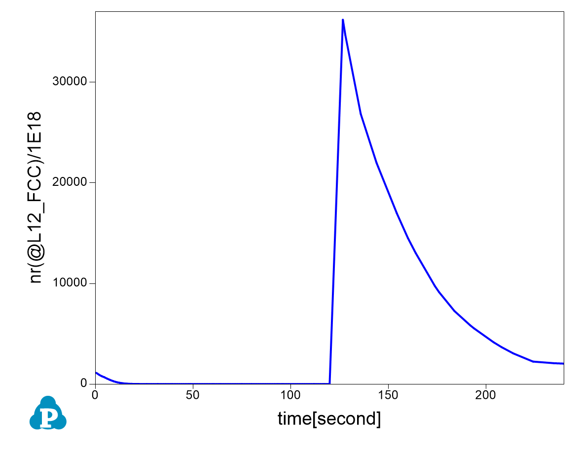
Figure 7. Time-evolution of nucleation rate of L12 phase